Using the Ornstein-Uhlenbeck Process for Random Exploration
Johannes Nauta, Yara Khaluf and Pieter Simoens
Department of Information Technology, Ghent University, Ghent, Belgium
Keywords:
Brownian Motion, Exploration, Ornstein-Uhlenbeck Process.
Abstract:
In model-based Reinforcement Learning, an agent aims to learn a transition model between attainable states.
Since the agent initially has zero knowledge of the transition model, it needs to resort to random exploration
in order to learn the model. In this work, we demonstrate how the Ornstein-Uhlenbeck process can be used as
a sampling scheme to generate exploratory Brownian motion in the absence of a transition model. Whereas
current approaches rely on knowledge of the transition model to generate the steps of Brownian motion, the
Ornstein-Uhlenbeck process does not. Additionally, the Ornstein-Uhlenbeck process naturally includes a drift
term originating from a potential function. We show that this potential can be controlled by the agent itself,
and allows executing non-equilibrium behavior such as ballistic motion or local trapping.
1 INTRODUCTION
In autonomous and complex systems, exploration is a
necessary component for learning how to act within
an unknown environment (Wilson et al., 1996). A
widely used approach wherein an agent aims to max-
imize a cumulative task specific reward is Reinforce-
ment Learning (RL). Specifically, model-based RL
includes an alternative (or additional) goal where the
reward is not only task specific but tied to learning the
transition model between attainable states. Once the
model is learnt, the agent can exploit this knowledge
to plan the most rewarding actions given a task, mak-
ing model-based learning approaches display gener-
alization capabilities. Since the agent has no prior
knowledge of the environment, it needs to resort to ex-
ploration to search and learn within the environment
before any exploitation can occur.
Essentially, efficient exploration is a search for
novelty, in which the agent should be steered towards
previously unvisited states. Model-based learning
benefits from efficient exploration because to gener-
ate a global transition model all states within the state
space first have to be visited. In model-based RL, the
novelty increases in sparsity as the agent visits more
of the state space. This essentially converts explo-
ration to a problem of sparse target search. Extensive
search for sparse targets via random walks is a widely
studied subject in the field of ecology (Viswanathan
et al., 1999; Bartumeus et al., 2005; Ferreira et al.,
2012). However, these approaches execute random
walks based on knowing the transition model. Since
the transition model is absent in novel environments,
these approaches are insufficient for use as an explo-
ration strategy. We therefore aim to use an efficient
exploration strategy that visits many different attain-
able states using random walks that do not require a
transition model.
As a first step, we wish to generate Brownian mo-
tion through action sampling. Arguably, while Brow-
nian motion as a search strategy is often outperformed
by other types of random walks, it is efficient in case
of revisitable targets (James et al., 2010) or in the
presence of a bias (Palyulin et al., 2014). Hence,
we consider action-driven Brownian motion as a step-
ping stone for further enhancing exploration in the
absence of a transition model. Random walks re-
sulting from action sampling have been described in
(Lillicrap et al., 2015), where similar to our work
the random walk is considered an exploration pol-
icy. However, their framework is not suitable for
model-learning as well as analytical expressions for
the agents’ movement are missing.
For a model-learning RL agent, executing Brow-
nian motion is non-trivial, because traditionally the
motion is achieved by sampling displacements from
a desired distribution. For example, in two dimen-
sions an angle and step-length are sampled and the
agent moves accordingly. However, when the tran-
sition model is unknown, the agent is unable to de-
termine the action that would result in this target dis-
placement, rendering such sampling procedures ob-
solete. We therefore introduce an action-sampling
framework based on the Ornstein-Uhlenbeck (OU)
Nauta, J., Khaluf, Y. and Simoens, P.
Using the Ornstein-Uhlenbeck Process for Random Exploration.
DOI: 10.5220/0007724500590066
In Proceedings of the 4th International Conference on Complexity, Future Information Systems and Risk (COMPLEXIS 2019), pages 59-66
ISBN: 978-989-758-366-7
Copyright
c
 2019 by SCITEPRESS – Science and Technology Publications, Lda. All rights reserved
59

process (Uhlenbeck and Ornstein, 1930). The OU
process allows an agent to realize Brownian motion
by sampling actions and without access to a transition
model. After convergence, the OU process evolves
the agents’ velocity according to a Langevin equation
with normally distributed random forces. The fact
that the agent’s velocity follows a Gaussian distribu-
tion, gives rise to the Brownian motion.
Additionally, the OU process naturally encom-
passes a drift term. This drift term can be formu-
lated such that it originates from self-induced poten-
tials by the agent. This allows the agent to change
to non-equilibrium motion, which holds promise for
replicating other types of random walks. Changing
the motion is a necessity for efficiency, since opti-
mal search often interchanges local Brownian mo-
tion with long-range displacements (Bartumeus et al.,
2005; Ferreira et al., 2012). Such active Brownian
motion has been studied in biology and physics (Ro-
manczuk et al., 2012), where active Brownian mo-
tion results in out-of-equilibrium motion through self-
propellation (Volpe et al., 2014; Basu et al., 2018).
The paper is organized as follows. We first char-
acterize random walks and discuss several metrics in
Section 2. Then, the OU process is described and ana-
lytical expressions for the metrics are obtained in Sec-
tion 3. We additionally introduce the internal drive
and generalize to higher dimensions. The sampling
procedure and numerical details are listed in Sec-
tion 4. Both analytical and empirical results acquired
through simulation are shown in Section 5. The paper
is concluded with a discussion in Section 6.
2 RANDOM WALKS FOR
EXPLORATION
Let us consider an agent as a particle within a Eu-
clidean space. Whereas the ultimate goal of the agent
is to learn a transition model that predicts the next
state given an action, this paper focuses on the frame-
work that generates random walks for exploration.
These need to satisfy a number of requirements. First,
the framework needs to be able to handle continuous
state and action spaces, since physical control tasks
are often continuous in both states and actions. Sec-
ond, in absence of a transition model, the framework
needs to be based on sampling actions. Third, the
framework needs to incorporate an intrinsic drive that
influences the motion of the agent. The OU process
incorporates all three requirements and is therefore an
excellent choice for use as an exploration strategy.
2.1 Metrics
Random walks are often characterized by several met-
rics, mainly the distribution of step-lengths as well
as the mean squared displacement. The step-length
distribution essentially determines the type of ran-
dom walk. Brownian motion is recovered when the
step-lengths are distributed according to a zero-mean
Gaussian. The mean squared displacement

R
2
(t)

of
the agent is an indication of the size of the explored
regions of the state space. In one dimension, the mean
squared displacement is given by

R
2
(t)

v
0
=

(x(t) − x
0
)
2

v
0
, (1)
where v
0
the velocity and x
0
the position at t = 0. The
operator
h
.
i
v
0
denotes the ensemble average, which
is computed by averaging over many non-interacting
agents that all start with the same initial velocity v
0
.
2.2 Coverage of the State Space
The time evolution of the mean squared displacement
is an indication of the efficiency of the coverage of
the random walk. It corresponds to different types of
diffusion, characterized by a power-law exponent γ,
where

R
2
(t)

v
0
∝ t
γ
, γ > 0 (2)
Normal diffusion has linear scaling of the mean
squared displacement with time, corresponding to
γ = 1. If γ < 1, the agent undergoes subdiffusion
and for γ > 1 superdiffusion arises. Since the mean
squared displacement is an indication of the explored
area of the environment, higher values of γ are gen-
erally preferred when the goal is to increase this cov-
erage. However, one should be careful when mak-
ing conclusions of the random walk based solely on
the time evolution of the mean squared displacement.
For example, ballistic (straight line) motion is easily
regained by simply evolving the agent according to
x = vt, with a constant velocity v. In this case, it is
simple to see that γ = 2. However, intuitively, ballistic
motion does not lead to a homogeneous coverage of
the explored environment and thus γ can give a wrong
indication of the movement of the agent and should
be interpreted with care.
3 THE ORNSTEIN-UHLENBECK
PROCESS
In this section, we introduce the reader to the OU
process that forms the foundation of the sampling
COMPLEXIS 2019 - 4th International Conference on Complexity, Future Information Systems and Risk
60

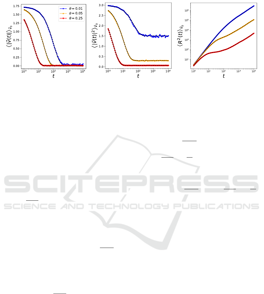
(a) Ensemble mean of velocity (b) Ensemble mean of squared velocity (c) Mean squared displacement
Figure 1: Ensemble averages of the first (a) and second (b) moments of the velocity for the three-dimensional OU process
with uncorrelated Brownian noise, for different values of θ. Mean square displacements of the same processes are shown in
(c). Note the convergence to γ ≈ 1 when t increases. In this case,~µ = (0,0, 0)
T
, ~v
0
= (1,1, 1)
T
, ~x
0
= (0,0, 0)
T
. Black dotted
lines indicate the analytical result.
scheme that is presented in Section 4. The OU pro-
cess is a well-known diffusion process described by a
Langevin equation (Uhlenbeck and Ornstein, 1930).
In one dimension, the position of the agent starting at
x
0
is given by
x(t) = x
0
+
Z
t
0
v(s)ds (3)
The velocity is derived from Newton’s law and has
the following form
m
dv(t)
dt
= −mθv(t) + F
U
(x) + B(t), (4)
where θ denotes a friction coefficient, F
U
(x) the ex-
ternal force and B(t) the stochastic force acting on
the agent with mass m. The ensemble average of the
velocity is given by
h
v(t)
i
v
0
= v
0
e
−θt
+ µ

1 − e
−θt

, µ =
F
U
(x)
mθ
(5)
which converges to the drift µ in the time limit t → ∞.
The second moment is given by

v
2
(t)

v
0
=
h
v
0
e
−θt
+ µ

1 − e
−θt
i
2
+
g
2θm
2

1 − e
−2θt

, (6)
where g is the correlation strength of the stochas-
tic forces, indicating a time-range over which the
stochastic forces are correlated. In the large-time
limit, the second moment equals µ
2
+ g/2θm
2
, given
that F
U
(x) = F
U
a constant. In contrast with the first
moment, this includes a dependency on the friction
coefficient θ in the large-time limit, generating an off-
set due to friction.
Next we wish to determine the mean squared dis-
placement of the ensemble in the presence of a con-
stant external force

R
2
(t)

v
0
=

v
0
− µ
θ

1 − e
−θt

+ µt

2
+
g
m
2
θ
2

t +
1
2θ

4e
−θt
− e
−2θt
− 3


, (7)
which in the large-time limit equals
lim
t→∞

R
2
(t)

v
0
=

v
0
− µ
θ
+ µt

2
+
g
m
2
θ
2

t −
3
2θ

(8)
When the drift equals 0 we obtain the famous result
of Einstein, namely that the mean squared displace-
ment scales linearly with time, i.e.

R
2
(t)

v
0
∝ t
(Einstein, 1905). When the drift is non-zero, we ob-
tain

R
2
(t)

v
0
∝ t
2
. Furthermore, v(t) is normally
distributed when t → ∞, with mean µ and variance

v
2
(t)

v
0
−
h
v(t)
i
2
v
0
. As a result, displacements of
the position x(t) are normally distributed, effectively
replicating Brownian motion when µ = 0.
3.1 Origin of Internal Drift
In physics, the drift µ is typically regarded as an ex-
trinsic effect, uncontrollable by the agent. However,
it is important to note that the sampling of the forces
(and thus the velocities) is performed by the agent
itself. Thus, applying an external drift to a passive
agent is the same as applying an internal drift to an
active agent. As motivated in the introduction, this in-
ternal drift can act similar to a curiosity signal (Hafez
et al., 2017), where the agent can undergo a drastic
transition or stay close to its current location depend-
ing on its intentions.
Using the Ornstein-Uhlenbeck Process for Random Exploration
61

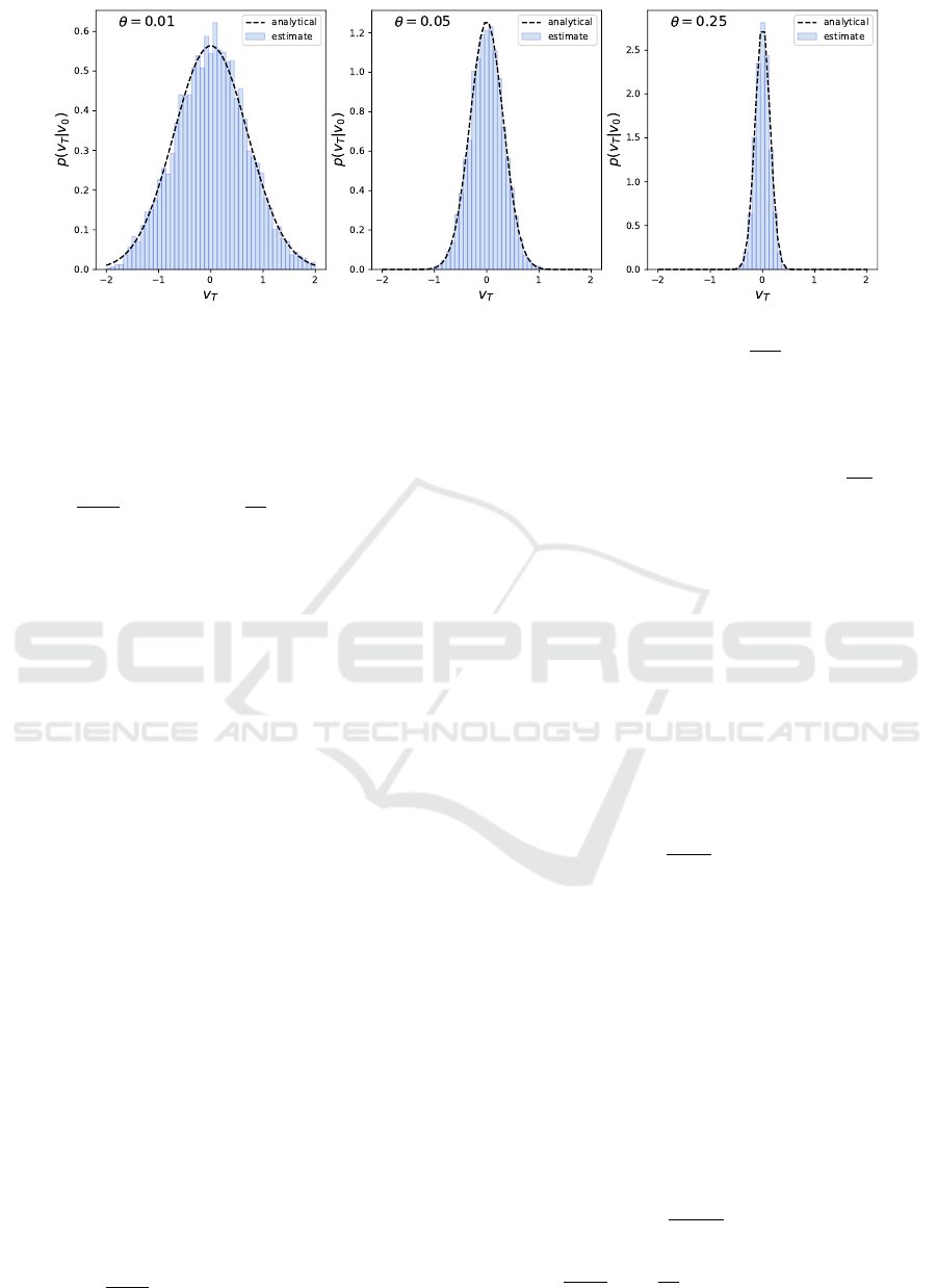
Figure 2: Velocity distributions for the one-dimensional OU process at T = n∆t, for different values of θ, µ = 0, v
0
= 1,m = 1.
Note that the distribution is Gaussian with mean
h
v(T )
i
v
0
= µ and variance

v
2
(T )

v
0
−
h
v(T )
i
2
v
0
=
g
2θm
2
.
Analytically, F
U
can be written as the derivative
of a potential U(x,t), giving us the Langevin equation
for the velocity as
m
dv(t)
dt
= −mθv(t) −
d
dx
U(x,t) + B(t), (9)
where the minus sign appears through the resulting in-
trinsic force F
U
= −dU/dx. This equation indicates
that the drift can be both position-dependent and time-
dependent. Note that the performed analysis to com-
pute the ensemble averages does only holds when the
potential is position-dependent, not time-dependent.
Since the velocity converges to µ = F
U
/mθ in the
large-time limit (see Eq. (5)), an agent can thus ac-
tively induce non-equilibrium behavior by manipulat-
ing the self-induced potential. For instance, an ap-
propriate choice of potential will allow the agent to
“trap” itself in a region or conversely to realize bal-
listic (straight line) motion. In the remainder of this
paper, we shall only consider position dependent po-
tentials.
3.2 Generalization to Multiple
Dimensions
In RL, action spaces are often high-dimensional. For
example, a robotic arm can have multiple joints on
which forces can be exerted. Therefore, if we wish to
enable model-based learning for agents with many de-
grees of freedom, we need to extend the OU process
to higher dimensions. This generalization is straight-
forward by considering the n-dimensional Langevin
equation
~x(t) =~x
0
+
Z
t
0
~v
s
ds, (10)
m
d~v(t)
dt
= −mθ~v(t) +
~
F
U
+
~
B(t), (11)
Solving the Langevin equation and computing the en-
semble average again gives
h
~v(t)
i
=~v
0
e
−θt
+~µ(1 − e
−θt
), ~µ =
~
F
U
mθ
(12)
When t → ∞, the ensemble average of the veloc-
ity again converges to the external drift ~µ since
for each dimension holds lim
t→∞
h
v
i
(t)
i
~v
0
= µ
i
.
The mean squared displacement depends on the
correlation matrix Σ
v(t)
. The random forces
are considered uncorrelated if the noise vector
~
B(t) = (B
1
(t),B
2
(t),. .. B
n
(t)) is an n-dimensional
vector consisting of independent Wiener processes
(Ibe, 2013), i.e.

B
i
(t)B
j
(t
0
)

= gδ
i j
δ(t −t
0
), (13)
where δ
i j
is the Kronecker delta and δ(t −t
0
) the Dirac
delta function. The covariance matrix of the velocity
is given by
Σ
v(t)
i j
=
gδ
i j
2θm
2

1 − e
−2θt

, (14)
which is a diagonal matrix. Thus our n-dimensional
velocity is distributed according to a multivariate
Gaussian distribution with mean ~µ and diagonal co-
variance matrix Σ
v(t)
. For computing the mean
squared displacement we define ~r(t) = ~x(t) −~x
0
,
which gives
R
2
(t) = |~r(t)|
2
=
n
∑
i=1
r
2
i
(t), (15)
which is simply the sum of the squared displacements
in each dimension (i.e. the square of the Euclidean
distance between~x(t) and~x
0
). Substituting the veloc-
ity of Eq. (11) and squaring we have

R
2
(t)

~v
0
=
n
∑
i=1

v
0
i
− µ
i
θ

1 − e
−θt

+ µ
i
t

2
+
gt
m
2
θ
2

t +
1
2θ
h
4e
−θt
− e
−2θt
− 3
i

, (16)
COMPLEXIS 2019 - 4th International Conference on Complexity, Future Information Systems and Risk
62

which is the sum of the mean squared displacement
in all dimensions, where each dimension has the same
expression as Eq. (7). This result is expected, since
we defined the n-dimensional noise vector having in-
dependent components. Therefore, each dimension is
undergoing Brownian motion, with the mean squared
displacement being the sum of displacements in each
dimension. Brownian motion is often modelled us-
ing correlated noise (i.e. non-diagonal elements of
the covariance matrix are non-zero), however careful
analysis of such systems are considered future work.
4 SAMPLING PROCEDURE
To realize Brownian motion in the state space S at
discretized points in time with time-steps ∆t, an agent
with mass m = 1 will sample forces ξ from a normal
distribution ξ with mean 0 and standard deviation ∆t,
N (0,∆t). This results in a time-discretization of Eq.
(10) and Eq. (11) of the velocity and position in each
dimension i:
v
t+∆t,i
= v
t,i
(1 − θ∆t) + µ
i
+ ξ
t,i
, (17)
x
t+∆t,i
= x
t,i
+ v
t+∆t,i
∆t (18)
Setting the standard deviation of ξ
t,i
to ∆t also de-
fines the correlation strength of stochastic driving
force, namely

B
2
(t)

= g = ∆t. This means that
the stochastic forces are only correlated within a time
range ∆t, defining a Wiener process. Ensemble aver-
ages of the (squared) velocity and the mean squared
displacement are computed over an ensemble of N =
1000 non-interacting agents, unless stated otherwise.
Since our interest lies mostly in the large-time limit,
we evolve Eq. (17) and Eq. (18) for n = 10
6
steps,
where ∆t = 0.01. In multiple dimensions, we com-
pute the ensemble average of the absolute value of the
velocity, i.e. the length of the velocity vector,
|~v(t)| =
s
D
∑
i=1
v
2
i
(t), |~v
2
(t)| =
D
∑
i=1
v
2
i
(t), (19)
where D is the number of dimensions. The power-law
exponent of the mean squared displacement can be
numerically approximated by discretizing time with
increments s:
γ(t) ≈
log


R
2
(t + s)

v
0

− log


R
2
(t)

v
0

log(t + s) − log(t)
, (20)
where log(·) the natural logarithm.
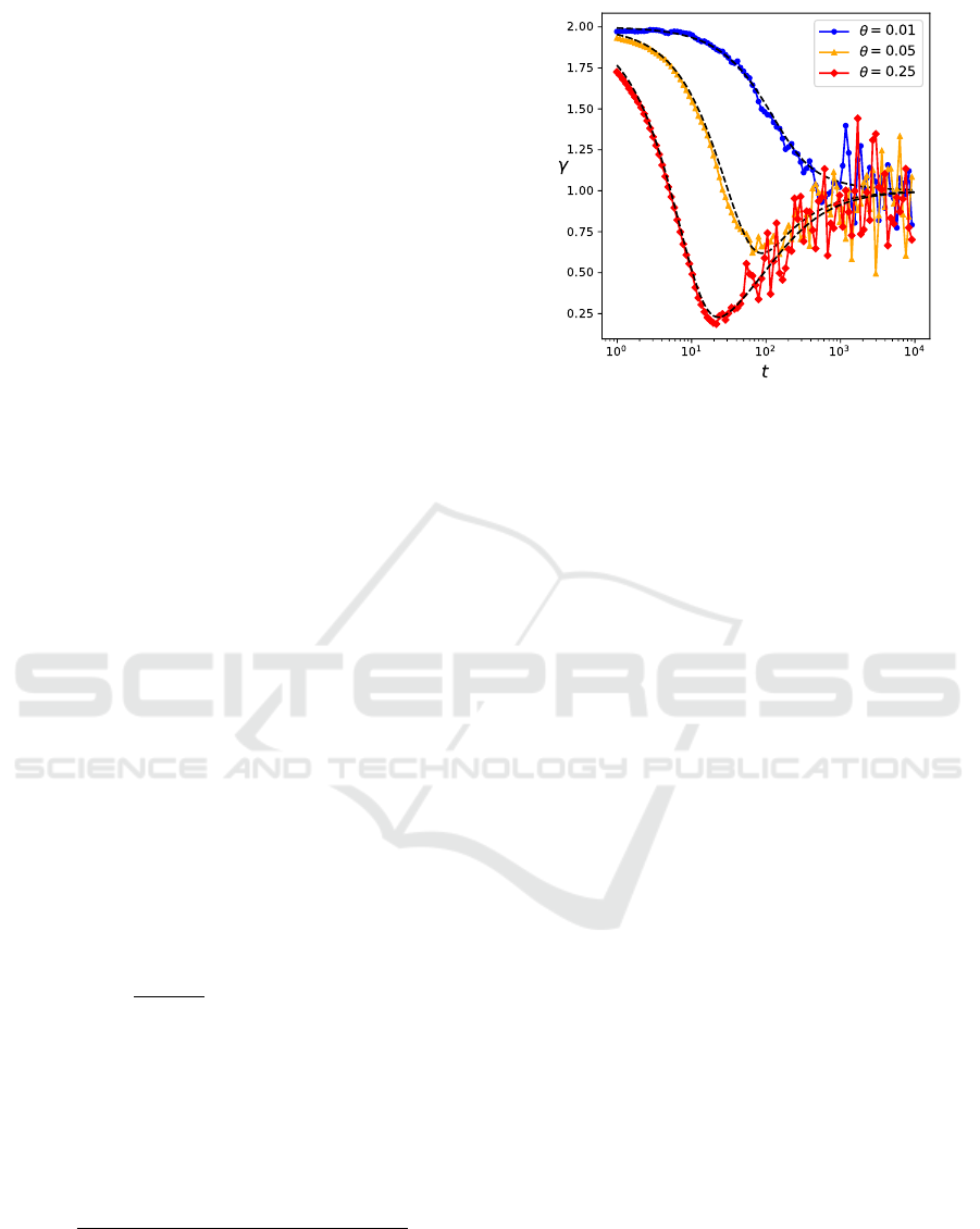
Figure 3: Power-law exponent γ of the three-dimensional
OU process with uncorrelated Brownian noise for µ = 0,
v
0
= 1, x
0
= 0. For large t, γ ≈ 1, indicating standard dif-
fusion, i.e. Brownian motion. Black dotted lines indicate
the analytical result. Note that at t → ∞, γ → 1 regardless
of θ. Large deviations are due to numerical computation of
the derivative.
5 RESULTS
We verify the analytical results and build upon the re-
sults to display active particle steering is able to ef-
fectively guide the agent to undergo non-equilibrium
behavior. In Section 5.1, we first validate whether we
are indeed able to realize Brownian motion through
action sampling. In Section 5.2, we show an agent
can change the distribution of the state space explo-
ration trajectory by applying different potentials.
5.1 Brownian Motion
We investigate the numerical simulations of the three-
dimensional OU process in the absence of a drift term
(µ = 0), described through Eqs. (17) and (18). We aim
to verify that each agent is indeed undergoing Brown-
ian motion through measuring the metrics mentioned
in Section 2.
5.1.1 Velocity Distribution
The velocity distribution is defined through the first
and second moment. The results for both moments
are displayed in Figs. 1a, 1b. Excellent agreement
between the analytical and numerical solutions is ob-
served. For large t, the first moment of the veloc-
ity tends towards the extrinsic drift µ = 0, whereas
the second moment converges to a value that depends
on θ. For both moments, the strength θ determines
Using the Ornstein-Uhlenbeck Process for Random Exploration
63

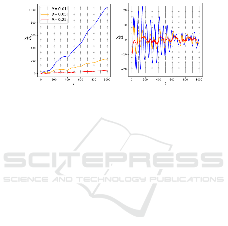
(a) (b)
Figure 4: Sample trajectories of the one-dimensional Brownian particle in different potentials for different strengths of the
OU process, for n = 10
5
steps, ∆t = 0.01. The arrows indicate the potential U(x). (a) U(x) = − ax, for x
0
= 0, a = 0.01,
(b) U(x) = ax
2
, for x
0
= −10, a = 0.01.
the convergence time of the process through a typi-
cal time τ = θ
−1
. In the large time limit, the velocity
is Gaussian (Uhlenbeck and Ornstein, 1930) around
µ = 0. This is indicated in Fig. 2, where the empirical
velocity at T = n∆t is indeed Gaussian. This means
that, for large t, the agent is sampling from a (multi-
variate) Gaussian.
5.1.2 Mean Squared Displacement
The mean squared displacement is plotted in Fig. 1c.
The analytical and numerical results are again in ex-
cellent agreement. The power-law coefficient of the
mean squared displacement, calculated by means of
Eq. (20), is plotted in Fig. 3. Note the transition be-
tween super-linear scaling (γ > 1) and linear scaling
(γ = 1) around the typical time τ = θ
−1
. Furthermore,
for large θ, there exists a time window of subdiffusion
(γ < 1) arising from the slowing down of the agents
due to a large friction coefficient θ.
5.2 Active Motion
Next we shall consider two elementary potential func-
tions U (x) to demonstrate how an agent can induce
other types of (non-equilibrium) motion. Ballistic
motion is able to induce large displacements, desired
if the agent wishes to visit far away regions of the state
space. In contrast, trapping the agent around a cer-
tain state enables local exploration where movement
is bound to a small area. Combining large displace-
ments and local trapping can give rise to continuous
time random walks (Volpe and Volpe, 2017). Addi-
tionally, the combination of these two potentials may
enable replication of many different continuous time
random walks, as these are often a combination of lo-
cal Brownian motion and long, correlated movement
(Zaburdaev et al., 2015). For visual purposes, we have
chosen to illustrate all results in one dimension, how-
ever generalization to multiple dimensions is trivial
(see Section 4).
5.2.1 Linear Potential
Let us consider a linear potential U = −ax such that
dv(t)
dt
= −θv(t) + a + B(t) (21)
A sample trajectory is shown in Fig. 4a. For lower
values of θ, the agent experiences less friction and
thus larger deviations are observed. This indicates the
trivial result that a frictionless particle exhibits higher
displacements within the same time. In the large-time
limit, we know that the ensemble mean of the veloc-
ity converges to the drift µ = a. The result is that the
Brownian particle will move with a close to constant
velocity when time increases (see Figs. 6a, 6b), re-
sulting in the visible straight line displacement with
respect to time as seen in Fig. 4. Thus, by using a lin-
ear potential, we are able to actively steer the agent to
undergo ballistic motion corresponding to x = vt with
a constant velocity µ = a/θ in the large time limit. As
shown in Fig. 5a, the mean squared displacement in-
deed evolves according to γ ≈ 2 for all θ when t is
large.
COMPLEXIS 2019 - 4th International Conference on Complexity, Future Information Systems and Risk
64

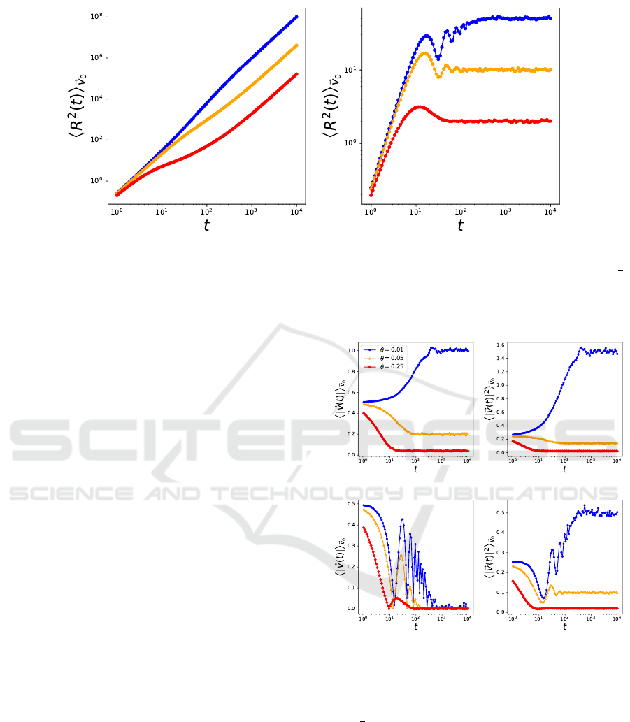
(a) Linear potential (b) Quadratic potential
Figure 5: Mean squared displacement of the OU process in different potentials, for different values of θ. Here, v
0
=
1
2
,
x
0
= 0, a = 0.01. (a) Given a linear potential U = −ax, we note that the mean squared displacement scales according to γ ≈ 2.
(b) Indicates trapping of the particle for U = ax
2
(γ = 0) where θ influences the average displacement at which the particle
becomes trapped.
5.2.2 Quadratic Potential
Let us consider a quadratic potential U = ax
2
such
that
dv(t)
dt
= −θv(t) − ax + B(t) (22)
By applying this potential, we expect that the agent
can trap itself close to the minimum of this poten-
tial at x = 0, with θ again describing the influence of
friction. High friction results in fast trapping of the
agent, whereas low friction indeed displays fluctua-
tions around the minimum of the potential with sig-
nificantly larger times necessary before effective trap-
ping occurs (see Fig. 4). For small θ, the agent is able
to drift further away from the minimum of the po-
tential due to overshooting the minimum. The mean
squared displacement is plotted in Fig. 5 for different
values of θ. After some time, the agent indeed be-
comes trapped, indicated by a stagnation of the mean
squared displacement and the mean velocity (see Figs.
5b, 6c). The friction coefficient of the OU process en-
codes deviations from the mean, meaning that small
values of θ indicate a higher variance for the velocity
distribution, as indicated in Fig. 6d. This induces, on
average, further displacements from the minimum of
the potential at x = 0. The first and second moments
of the velocity converge to different values for differ-
ent θ.
(a) (b)
(c) (d)
Figure 6: Ensemble average of first and second moments of
the velocity for the one-dimensional OU process in different
potentials, for different values of θ. Colours corresponding
to different θ are shown in the legend in (a). In all cases,
v
0
=
1
2
, x
0
= 0, a = 0.01. a) + (b): Linear potential U =
−ax. (c) + (d): Quadratic potential, U = ax
2
.
6 CONCLUSION
Learning a state transition model is a prerequisite of
any model-based RL control paradigm. To learn such
a model efficiently, an agent must efficiently explore
the state space. In this paper, we presented an ap-
Using the Ornstein-Uhlenbeck Process for Random Exploration
65

proach that is based on the OU process to realize ac-
tive guidance of an agent through state space by sam-
pling velocities instead of displacements. We have as-
sumed zero knowledge of the transition model, since
this is generally the case in most model-based RL set-
tings. The OU process evolves the agents’ velocity
according to a Langevin equation, where in the large-
time limit the sampled velocities follow a Gaussian
distribution. Additionally, the model allows the agent
to influence the action sampling scheme (and thus its
motion pattern) by means of a self-induced potential
function. One key advantage of our approach is that
we can derive closed-form analytical expressions.
In this paper, we have assumed that the transi-
tion model remains unknown, even after the agent has
explored the environment for some time. However,
when model-based learning is considered, the agent
often builds its knowledge in a incremental, iterative
fashion. In order to account for this, in future work we
will study the effects of making the strength θ time-
dependent as well as changing the intrinsic drift term
µ in reaction to encountered novelty. This generates a
framework wherein the intrinsic drive originates from
extrinsic sources or observations, resembling an intu-
itive implementation of a curious agent.
Furthermore, acquiring similar analytical expres-
sions for different types of random walks is highly de-
sirable. In particular, we wish to focus on a L
´
evy walk
(Zaburdaev et al., 2015). In a L
´
evy walk, the displace-
ments are sampled from a power law, interchang-
ing local displacements with long time-correlated dis-
placements within the environment. Using different
potentials, one can most likely replicate L
´
evy-like be-
havior through the process described in this work.
One could alternatively use a different formulation
of the underlying noise scheme, i.e. sample directly
from the desired distribution. This possibly give rise
to L
´
evy walks and might further enhance exploration
of an environment (Bartumeus et al., 2005; Ferreira
et al., 2012).
This work indicates a stepping stone in simulat-
ing random walks for exploration. Enabling random
walks in the absence of a transition model might
prove beneficial for model-based RL, even opening
the doors to more efficient sampling schemes that im-
prove learning in continuous state spaces.
REFERENCES
Bartumeus, F., da Luz, M. G. E., Viswanathan, G. M., and
Catalan, J. (2005). Animal search strategies: a quan-
titative random-walk analysis. Ecology, 86(11):3078–
3087.
Basu, U., Majumdar, S. N., Rosso, A., and Schehr, G.
(2018). Active brownian motion in two dimensions.
arXiv preprint arXiv:1804.09027.
Einstein, A. (1905). Investigations on the theory of the
brownian movement. Ann. der Physik.
Ferreira, A., Raposo, E., Viswanathan, G., and da Luz, M.
(2012). The influence of the environment on l
´
evy ran-
dom search efficiency: Fractality and memory effects.
Physica A: Statistical Mechanics and its Applications,
391(11):3234 – 3246.
Hafez, M. B., Weber, C., and Wermter, S. (2017). Curiosity-
driven exploration enhances motor skills of continu-
ous actor-critic learner. In 2017 Joint IEEE Interna-
tional Conference on Development and Learning and
Epigenetic Robotics (ICDL-EpiRob), pages 39–46.
Ibe, O. C. (2013). Elements of Random Walk and Diffusion
Processes. Wiley Publishing, 1st edition.
James, A., Pitchford, J. W., and Plank, M. (2010). Efficient
or inaccurate? analytical and numerical modelling of
random search strategies. Bulletin of Mathematical
Biology, 72(4):896–913.
Lillicrap, T. P., Hunt, J. J., Pritzel, A., Heess, N., Erez, T.,
Tassa, Y., Silver, D., and Wierstra, D. (2015). Contin-
uous control with deep reinforcement learning. CoRR,
abs/1509.02971.
Palyulin, V. V., Chechkin, A. V., and Metzler, R. (2014).
L
´
evy flights do not always optimize random blind
search for sparse targets. Proceedings of the National
Academy of Sciences, 111(8):2931–2936.
Romanczuk, P., B
¨
ar, M., Ebeling, W., Lindner, B., and
Schimansky-Geier, L. (2012). Active brownian par-
ticles. The European Physical Journal Special Topics,
202(1):1–162.
Uhlenbeck, G. E. and Ornstein, L. S. (1930). On the theory
of the brownian motion. Phys. Rev., 36:823–841.
Viswanathan, G. M., Buldyrev, S. V., Havlin, S., Da Luz,
M., Raposo, E., and Stanley, H. E. (1999). Op-
timizing the success of random searches. Nature,
401(6756):911.
Volpe, G., Gigan, S., and Volpe, G. (2014). Simulation
of the active brownian motion of a microswimmer.
American Journal of Physics, 82(7):659–664.
Volpe, G. and Volpe, G. (2017). The topography of the en-
vironment alters the optimal search strategy for active
particles. Proceedings of the National Academy of
Sciences, 114(43):11350–11355.
Wilson, S. W. et al. (1996). Explore/exploit strategies in
autonomy. In Proc. of the Fourth International Con-
ference on Simulation of Adaptive Behavior: From
Animals to Animats, volume 4, pages 325–332.
Zaburdaev, V., Denisov, S., and Klafter, J. (2015). L
´
evy
walks. Reviews of Modern Physics, 87(2):483.
COMPLEXIS 2019 - 4th International Conference on Complexity, Future Information Systems and Risk
66