
A Modified Self-training Method for Adapting Domains in the Task of
Food Classification
Elnaz Jahani Heravi
1
, Hamed H. Aghdam
2
and Domenec Puig
1
1
Department of Computer Engineering and Mathematics, University Rovira i Virgili, Spain
2
The Computer Vision Center, University Autonoma Barcelona, Spain
Keywords:
Domain Adaptation, Deep Learning, Food Recognition.
Abstract:
Food trackers are tools that recognize foods using their images. In the core of these tools there is usually
a neural network that performs the classification. Neural networks are highly expressive models that need a
large dataset to generalize well. Since it is hard to collect a training set that captures most of realistic situations
in real world, there is usually a shift between the training set and the actual test set. This potentially reduces
the performance of the network. In this paper, we propose a method based on self-training to perform unsu-
pervised domain adaptation in the task of food classification. Our method takes into account the uncertainty
of predictions instead of probability scores to assign pseudo-labels. Our experiments on the Food-101 and the
UPMC-101 datasets show that the proposed method produces more accurate results compared to Tri-training
method which had previously surpassed other domain adaptation methods.
1 INTRODUCTION
In the past few years, methods based on deep neu-
ral networks have the significantly improved perfor-
mance of different computer vision tasks such as clas-
sification, detection, and segmentation. This progress
became possible mainly for three reasons. First, pa-
rallel computing hardware and related software libra-
ries were emerged and made it possible to imple-
ment heavily computational models on these devices
in which running a large network on medium size
image takes less than a second. Second, large data-
sets such as ImageNet became available which were
composed of diverse samples. Using these large data-
sets, we were able to train larger networks with mil-
lions of parameters. Third, neural networks were ra-
pidly improved by the advent of ideas such as weight
sharing, initialization, micro-architectures, activation
functions, normalization, regularization, and optimi-
zation algorithms.
In general, the success of deep learning based met-
hods has been limited to applications where there is a
large dataset of diverse samples. However, neural net-
works might not generalize properly when they are
trained on datasets of few samples. This is due to
the fact that a neural network is a highly nonlinear
function and it is usually formulated using thousands
or millions of parameters. When there is not an ade-
quate amount of samples in a database, current trai-
ning algorithms cause the network to overfit on data
and it is very likely not to generalize well on test data.
Even if a network is trained using a large dataset,
it is probable that the network is overfitted on the da-
taset and it might not generalize well on the test set.
This is due to a phenomenon called database shift.
The aim of domain adaptation techniques is to train
models that are tolerant to shift in databases. In con-
tinuous domain adaptation setting, the classification
model is trained on a source dataset. Then, it is de-
ployed and eventually, new unlabeled data is added to
the database. The newly added samples (or some of
them) might be retained for the future, or they might
be removed from the database.
In order to do continuous domain adaptation, we
first need to study domain adaptation techniques in a
non-continuous setting in which there is a source da-
tabase and an unlabeled target database. This way,
we will be able to have a better understanding of the
advantages and disadvantages of each technique ta-
king into account the continuous domain adaptation
setting.
In this paper, we will formally explain the domain
adaptation problem in Section 2 and review state-of-
the-art methods in Section 3. Then, we propose a new
method in Section 4 by modifying the self-training
method and taking into account the uncertainty of pre-
Heravi, E., Aghdam, H. and Puig, D.
A Modified Self-training Method for Adapting Domains in the Task of Food Classification.
DOI: 10.5220/0007688801430154
In Proceedings of the 14th International Joint Conference on Computer Vision, Imaging and Computer Graphics Theory and Applications (VISIGRAPP 2019), pages 143-154
ISBN: 978-989-758-354-4
Copyright
c
2019 by SCITEPRESS – Science and Technology Publications, Lda. All rights reserved
143

diction rather than the probability scores. This makes
our method more tolerant to error reinforcement. Our
experiments on the Food-101 and the UPMC-101 da-
tasetts in Section 5 show that our method is able to
produce superior results compared to the recently pro-
posed approach based on tri-training.
2 FORMULATION
Assume the problem of training a neural network
for classifying some foods worldwide. To this end,
we need to collect a database of foods and manu-
ally label them. Denoting the database by X
s
=
{(x
0
s
, y
0
s
), . . . , (x
n
s
, y
n
s
)}, our aim is to train the classi-
fication model
g(x
s
) : R
H×W
→ R (1)
to predict the label of the input image. The database
could be created by only collecting images of food
from the Internet. Also, online users tend to decorate
a food and take the best shot. The database could be
collected considering different environmental condi-
tions, variations of the same food from one country to
another and the imaging devices.
Our goal is to train a food classification network
using these images. Then, we will deploy our mo-
del on a device which is designed to classify image
foods captured by the device. In other words, there is
another database called X
t
= {(x
0
t
, y
0
t
), . . . , (x
m
t
, y
m
t
)}
indicating the samples captured by the device. Here,
our dataset collected from the Internet is the source
domain and the dataset collected by the device is the
target domain where the actual test will take place.
Collecting X
s
using the first approach can be done
quickly and efficiently. In contrast, collecting X
s
using the second approach is hard and it is almost in
fact impractical. However, samples in the second ap-
proach will be diverse as opposed to the samples in
the first approach. Consequently, the model trained
on the second approach is likely to be more accurate
than the first approach. (Torralba and Efros, 2011)
showed in most cases there is a shift between X
s
and
X
t
even when X
s
is collected using the second appro-
ach. This shift between the databases negatively af-
fects the classification accuracy on X
t
.
More formally, the classification model g(x
s
) can
be formulated by the composite function g(x
s
) =
f (h(x
s
)) where h : R
H×W
→ X
D
is a function that
maps the input image into a D-dimensional space cal-
led feature space. The joint probability of vectors
in the feature space and their corresponding labels
are denoted by p
s
(h(x
s
), y
s
), and p
t
(h(x
t
), y
t
) for the
source domain and target domain, respectively.
Domain adaptation refers to the problem of trai-
ning the model f (h(x
s
)) when p
s
(h(X
s
)) 6= p
t
(h(X
t
))
but y
t
, y
s
∈ L where L is the label space. In other
words, domain adaptation assumes that the labels y
s
and y
t
are drawn from the common label space L and
h(x
s
) and h(x
t
) are also drawn from the common fea-
ture space X
D
. However, distribution of feature vec-
tors in the source domain is different from the distri-
bution of feature vectors in the target domain. This is
called covariate shift.
This is different from knowledge adaptation
where the basic assumption is that p
s
(h(X
s
)) '
p
t
(h(X
t
)) but y
s
∈ L and y
t
∈ L
0
are two different la-
bel spaces. Here, we have only focused on methods
for dealing with the covariate shift problem.
2.1 Domain Adaptation Types
Domain adaptation can be further divided into su-
pervised, unsupervised and semi-supervised domain
adaptation. In supervised domain adaptation, both X
s
and X
t
are labeled. In contrary, unsupervised dom-
ain adaptation deals with situations where the source
domain is labeled but the target domain is only com-
posed of h(x
t
) and y
t
is unknown for all target sam-
ples. Finally, semi-supervised domain adaptation re-
fers to problems where the target dataset is partially
labeled. However, the number of labeled target sam-
ples is very low. Figure 1 shows these three problems
schematically.
Unsupervised and semi-supervised domain adap-
tation has important practical applications. We ex-
plain one of these applications using an example. In
order to collect X
s
in our application, we can simply
rely on online images instead of collecting a diverse
range of food images from wall-mounted cameras in
real-world. This way, we can collect a considerable
amount of food images in a reasonable time.
Then, we can collect many images from a wall-
mounted camera in real-world without annotating
their labels and create the X
t
dataset. Finally, our mo-
del can be trained using both X
s
and X
t
. Using X
s
the model will learn essential visual clues that are re-
quired for classifying foods. Then, it will refine its
knowledge using the images in X
t
.
3 RELATED WORK
In this section, we will explain state-of-the-art domain
adaptation techniques that are applicable to the neu-
ral networks. Generally speaking, domain adaptation
techniques break down to feature space alignment, re-
construction based, generative adversarial networks
VISAPP 2019 - 14th International Conference on Computer Vision Theory and Applications
144
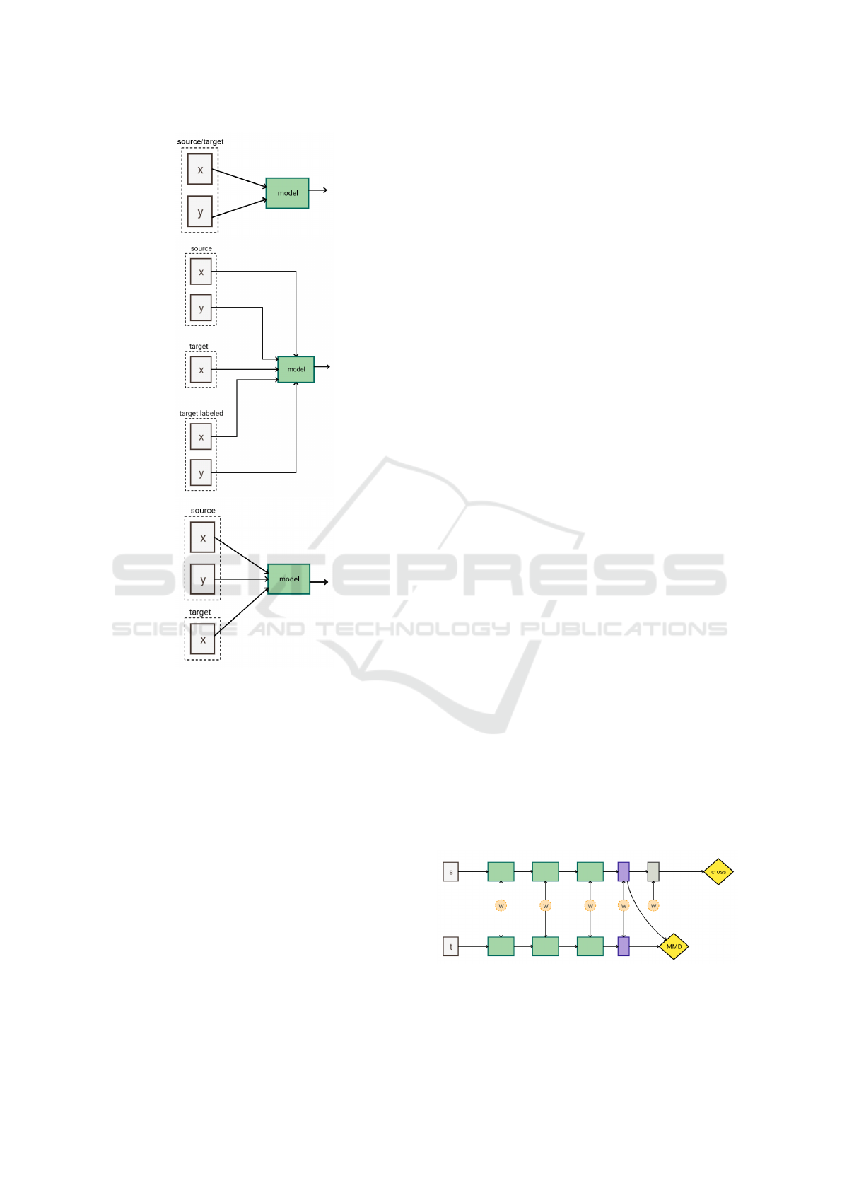
Figure 1: First to the third rows: supervised, semi-
supervised and unsupervised domain adaptation problems.
and semi-supervised learning.
3.1 Feature Space Alignment
Feature space alignment methods (Fernando et al.,
2013) directly manipulate the feature spaces such that
they are both aligned. The correlation alignment (Sun
et al., 2015; Wang et al., 2017; Morerio et al., 2017)
finds a linear transformation matrix A such that Ah(x
s
)
is aligned with h(x
t
). The transformation matrix A is
found by minimizing:
argmin
A
k A
T
C
s
A −C
t
k
2
F
(2)
where C
s
and C
t
are correlation matrices of the source
and target domains, respectively. Denoting mean sub-
tracted representation matrices with H
s
and H
t
, the
above equation will be equal to:
argmin
A
k A
T
H
T
s
H
s
A − H
T
t
H
t
k
2
F
. (3)
The advantage of the above formulation is that it is
a convex optimization problem. However, the main
drawback of this method is that all layers in the model
f (h(x)) are fixed during minimization of the above
objective function. To overcome this problem, (Bou-
smalis et al., 2016b) proposed to directly adapt all lay-
ers in h(x) by minimizing:
argmin
θ
k H
T
s
H
s
− H
T
t
H
t
k
2
F
. (4)
where θ denotes all parameters of h(x). On the one
hand, a neural network is normally trained using mini-
batches. On the other hand, h(x) is normally a high
dimensional vector. Consequently, small number of
samples in a mini-batch might not be able to accu-
rately approximate the correlation matrices. As the
result, the feature spaces will not be aligned properly.
3.1.1 Maximum Mean Discrepancy
Maximum Mean Discrepancy (MMD) is a method for
comparing two probability distributions (Tzeng et al.,
2014; Csurka et al., 2017; Shaham et al., 2016). It
achieves this goal by computing:
MMD(X
s
, X
t
) =
∑
x
s
,x
0
s
∈X
s
K (x
s
, x
0
s
) − 2
∑
x
s
∈X
s
∑
x
t
∈X
t
K (x
s
, x
t
) +
∑
x
t
,x
0
t
∈X
t
K (x
t
, x
0
t
)
(5)
where K is the kernel function. The above function
will be zero for perfectly aligned feature spaces. More
specifically, feature space represented by h(x) con-
stantly changes during training of a neural network
or aligning feature spaces by minimizing the above
objective function. Figure 2 shows the schematic dia-
gram of domain adaptation by minimizing the MMD
loss. The overall loss function is:
E = crossentropy(X
s
) + λMMD(X
s
, X
t
) (6)
It first starts with training the neural network using
only the cross-entropy loss (ie. λ = 0) on the source
domain for n iterations. Then, the network is minimi-
zed using both losses. (Long et al., 2015; Long et al.,
2016) computed MMD for different layers in addition
to the last layer. For example, Figure 3 shows how to
align feature spaces by minimizing MMD of two dif-
ferent layers.
Figure 2: Schematic diagram of domain adaptation
using MMD. Dashed circles show parameters of a layer.
Green/purple rectangles are analogous to convolution-
pooling/fully-connected layers.
A Modified Self-training Method for Adapting Domains in the Task of Food Classification
145
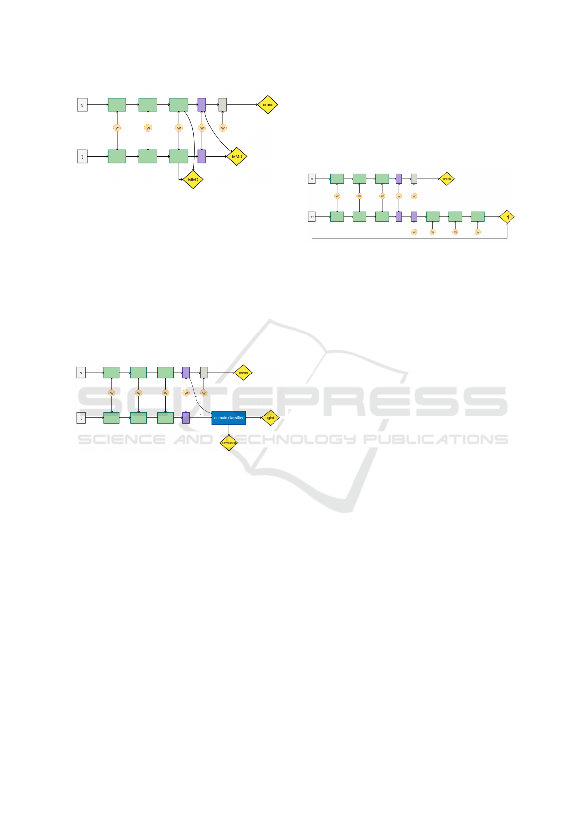
Figure 3: Schematic diagram of domain adaptation by com-
puting MMD for different layers.
3.1.2 Adversarial
Both Correlation Alignment and MMD methods di-
rectly align feature spaces. Domains can be also alig-
ned using an adversarial training technique. (Ganin
and Lempitsky, 2014; Ganin et al., 2015) first trained
a classifier to discriminate h(x
s
) from h(x
t
). Then,
they adapted h(x) by using the modified loss function
of the domain classifier. Figure 4 illustrates the sche-
matic diagram of domain adaptation using adversarial
training. Formally, the network is trained by minimi-
Figure 4: Schematic diagram of domain adaptation using
adversarial training.
zing the following objective functions (Tzeng et al.,
2017):
argmin
θ
h
,θ
f
crossentropy( f (h(X
s
)))
argmin
θ
d
−log
d(h(X
s
))
− log
1 − d(h(X
t
))
argmin
θ
h
−log
d(h(X
t
)
(7)
The first loss function is the common cross entropy
loss function. The second loss function is the logistic
loss for training the domain classifier. The third loss
function is the adversarial loss which adjusts parame-
ters of h() such that h(x
s
) is indistinguishable from
h(x
t
) by the domain classifier D(.). Instead of this
adversarial loss, (Tzeng et al., 2015) proposed cross
entropy loss using the uniform distribution. Advers-
arial domain adaptation has some challenges of Ge-
nerative Adversarial Networks (GANs) (Goodfellow
et al., 2014).
3.2 Reconstruction Based
In this approach, a decoder is attached to the encoder
of the neural network and the network tries to classify
source samples X
s
and reconstruct target samples X
t
.
Figure 5 shows the schematic diagram of this method.
Figure 5: Schematic diagram of domain adaptation using
reconstruction based methods.
In this method, the network is adapted by minimi-
zing:
argmin
θ
h
,θ
f
,θ
r
crossentropy( f (h(X
s
))) + (1 − λ)||
ˇ
X
t
− r(h(
ˆ
X
t
))||
2
(8)
where
ˇ
X
t
is degraded version of X
t
and r(h(
ˆ
X
t
)) is the
reconstructed image (Ghifary et al., 2016). The net-
work is first trained using only the cross entropy loss
function for n
1
iterations. Then, it is trained using
only the second term in the above loss function for
n
2
iterations. This process is repeated until meeting
the stopping criteria. The basic idea behind this met-
hod is that the reconstruction function r(h(
ˆ
X
t
)) learns
to reconstruct a degraded input. This way, given the
source sample x
s
, it will try to reconstruct h(
ˆ
X
s
) such
that it looks like a sample from X
t
.
3.3 Generative Adversarial Networks
Methods based on feature space alignment has an
important issue. Specifically, they try to minimize
the distance between marginal distributions p(X
s
) and
p(X
t
) ignoring the influence of the labels on these dis-
tributions.
The idea behind domain adaptation using Ge-
nerative Adversarial Networks (GANs) (Goodfellow
et al., 2014; Creswell et al., 2017) is to reduce the
divergence between X
s
and X
t
in image domain rat-
her than feature space. We explain the general idea
in Figure 6. In this method, we first train a GAN
to transform the given sample x
s
∈ X
s
to x
0
s
such that
x
0
s
possess similar visual properties of samples in X
t
which makes it indistinguishable from samples in X
t
(Bousmalis et al., 2016a). This transformation is done
using function G : R
H×W
→ R
H×W
.
After training the function G, a new dataset is
generated by applying this function to every sample
in X
s
. Then, the classification model is trained on
VISAPP 2019 - 14th International Conference on Computer Vision Theory and Applications
146
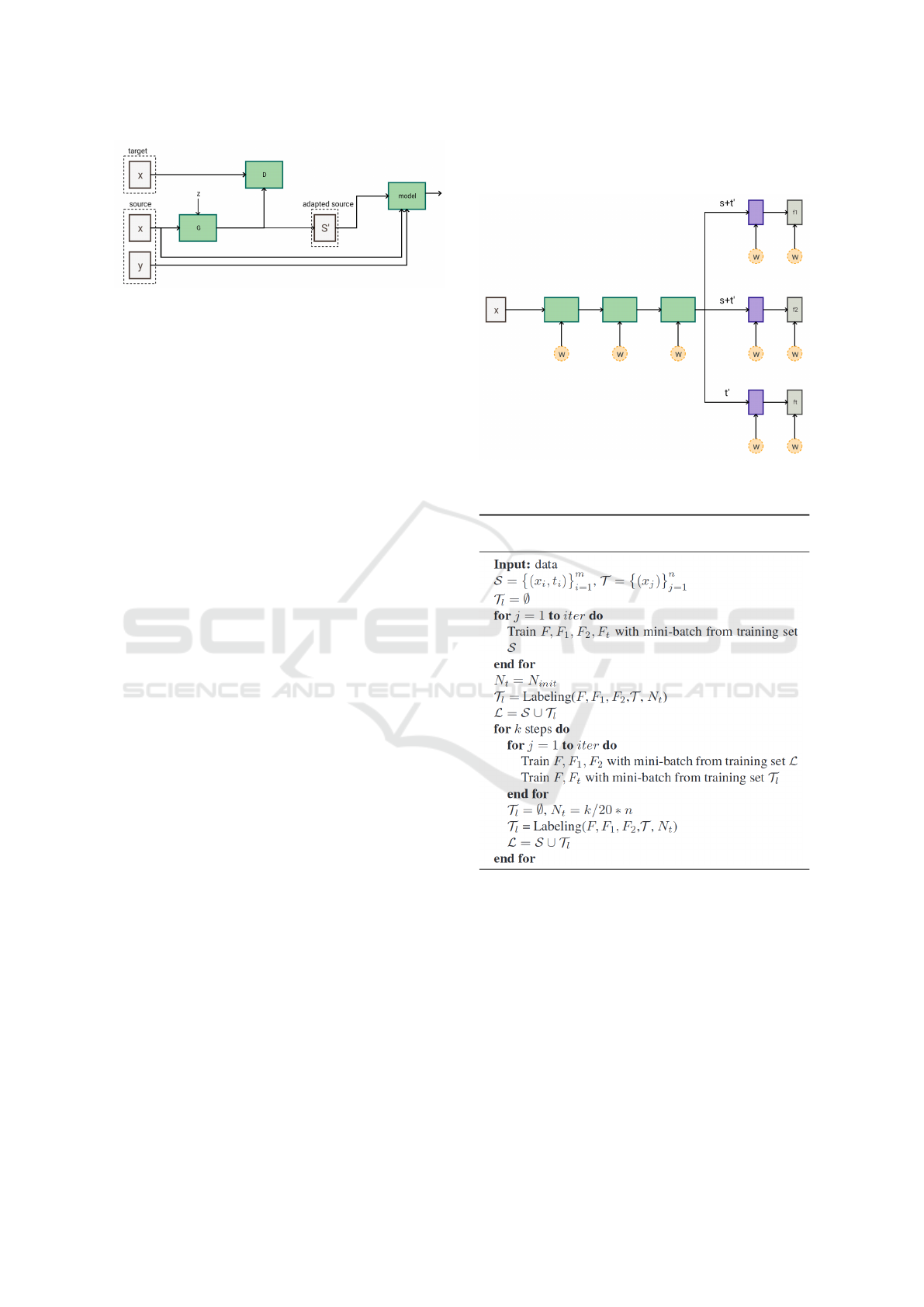
Figure 6: General idea behind domain adaptation using
GANs.
the adapted samples. Instead of training one GAN,
(Liu and Tuzel, 2016) trained two separate GANs
with shared weights on X
s
and X
t
. Also, (Hoffman
et al., 2017) trained a GAN using cycle consistent loss
which is able to adapt low-level visual cues as well.
This approach is intuitive and it decouples domain
adaptation from classification. The main challenge in
this approach is to design and train a GAN which is
able to accurately adapt samples from X
s
to X
t
.
3.4 Semi-supervised
Co-training is an approach in which two different
classifiers F
1
and F
2
with the common feature trans-
formation function h are trained on X
s
(Saito et al.,
2017). This way, there are two classifiers F
1
(h(x
s
))
and F
2
(h(x
s
)) which are both able to correctly clas-
sify x
s
but each of them has a different view on the
transformed feature h(x
s
). These two different views
are used for labeling some samples in X
t
based on a
few criteria. Then, the pseudo-labeled samples from
X
t
are combined with X
s
, and they are used for re-
fining F
1
and F
2
. This process is repeated until the
algorithm converges.
In contrast to reconstruction based methods or fe-
ature space alignment methods, this approach aligns
the feature spaces using pseudo labeled target sam-
ples. This actually aligns classes as opposed to the
adversarial domain adaptation methods. In addition,
this method does is easy to implement and train. Fi-
nally, it has also an analogy to the methods in (Haeus-
ser et al., 2017) which has proposed a loss function
based on the random walk on the bipartite graph.
Tri-training (Saito et al., 2017) is a variant of co-
training and it is a branch of a broader topic called
Multiview learning. In addition to F
1
and F
2
that we
explained above, Tri-training includes additional clas-
sifier F
T
which is explicitly trained to perform well on
the target dataset. In fact, the pseudo-labeled dataset
¯
X
t
produced using the above approach is used for trai-
ning the target classifier F
T
(h( ¯x
t
)). Figure 7 illustra-
tes the schematic diagram of this approach. Further-
more, Algorithm 1 explains the training algorithm of
Tri-training.
Figure 7: Schematic diagram of domain adaptation using
tri-training.
Algorithm 1: Tri-training algorithm for domain adaptation
(Saito et al., 2017).
The labeling step in this algorithm, assign pseudo
labels to target samples. A pseudo-label is assigned
to the unlabeled target sample x
t
if:
• argmax( f
1
(h(x
t
))) = argmax( f
2
(h(x
t
)))
• f
1
(h(x
t
)) > T or f
2
(h(x
t
)) > T
hold true. In other words, if both classifiers agree on
the class label of x
t
and confidence of one of them is
greater than T , a pseudo-label is assigned to the tar-
get sample x
t
. The confidence threshold value could
be set to 0.9 or 0.95. At each labeling operation, all
previously pseudo-labeled samples are removed from
the training. Then, N
t
samples are selected randomly
A Modified Self-training Method for Adapting Domains in the Task of Food Classification
147
from the target dataset and they are labeled according
to the above procedure. The number of selected sam-
ples N
t
is increased at each cycle of adaptation.
One important step in tri-training is to encourage
F
1
(h(x
s
)) and F
2
(h(x
s
)) to learn different representa-
tions. Denoting the weights of F
1
by w
1
and the weig-
hts of F
2
by w
2
, tri-training adds |w
1
· w
T
2
| to the loss
function to encourage the weights of the two bran-
ches to be orthogonal. The trivial solution for this
regularization term is that at least one of the weights
to be zero. However, the cross entropy loss attached
to each of these branches prevent the trivial solution.
Consequently, this term encourages the two branches
to learn different representations.
Tri-training has shown superior results in some
tasks compared to other methods explained in this pa-
per (Saito et al., 2017). However, this comes with the
cost of training two more branches. In addition, set-
ting the weak penalization of the regularization term
|w
T
1
· w
T
2
| will result in two classifiers which are not
basically different. In contrast, strong penalization
may encourage the trivial solution for the regulariza-
tion term |w
1
·w
T
2
|. This issue becomes more challen-
ging if we would like to train a network on a source
and target domain with a great divergence.
4 PROPOSED METHOD
Tri-training and co-training are in fact a variant of
another method called self-training. In self-training
(Ruder and Plank, 2018), instead of training two or
three different branches, we train a network with only
one classification branch and assign pseudo-labels to
the target samples if the prediction probability is gre-
ater than a threshold.
Self-training is faster to perform compared to Tri-
training. Yet, it suffers from a phenomenon called
error reinforcement. To be more specific, if the di-
vergence between the two domains is high, it is likely
that some target samples are incorrectly classified by
the network. This will cause that wrong labels are as-
signed to these samples. When they are added to the
training set, the number of samples with noisy labels
will increase in the training set.
This may potentially cause the network to learn
incorrect mapping. When the network is applied to
the target samples again, it may classify more samples
incorrectly. Hence, the error is likely to be reinforced
as more cycles of pseudo-labeling are performed.
Tri-training reduces this effect using two classi-
fiers with different views. Then, it selects samples
that both models agree with the class of the sample
and at least one of them produces a high probability.
From another perspective, Tri-training could be
seen as an ensemble of two models in which pseudo
labels are assigned by analyzing the ensemble. We
can combine the characteristics of the self-training
and tri-training and come up with a method that is
fast to perform and it is more tolerant against error
reinforcement. To this end, we propose the variant of
self-training indicated in Algorithm 2.
Algorithm 2: Proposed variant of self-training using pool of
multi-crop samples.
Θ: A neural network
X
s
: The source dataset
X
t
: The target dataset
K: An integer showing the number of samples for
evaluation at each cycle
Train Θ on X
s
for t = 1 : T do
X
t
0
: Select K samples randomly from X
t
X
s
0
= X
s
for x
t
0
∈ X
t
0
do
Evaluate x
t
0
using multi-scale multi-crop
validation with flipping
mi = Compute the mutual information x
t
0
if mi < threshold then
X
s
0
= X
s
S
x
t
0
Update Θ using X
s
0
K = αK (α > 1)
The algorithm starts with training the network on
the source domain. Then, it performs T cycles of
pseudo labeling. At each cycle, it randomly selects
K unlabeled samples from the target domain and eva-
luate each sample using the multi-crop, multi-scale
evaluation with flipping.
To be more specific, we set the size of each crop
to (s
h
×H, s
w
×W ) for an image of size H ×W where
s
h
, s
w
∈ [0, 1]. The first crop is obtained by placing
the cropping rectangle in the top left corner. Simi-
larly, the three other crops are obtained by placing the
cropping rectangle on the other four corners. The last
crop is obtained by placing the crop window at the
center. This way, five crops are generated. We gene-
rate a pool of 15 crops using crop sizes (0.9H, 0.9W ),
(0.8H, 0.8W ) and (0.7H, 0.7W ). Then, we add their
mirrored version to the pool. This way, the size of
the pool increases to 30 crops. Finally, we add the
original image and its mirrored version to the pool.
The Tri-training method assign pseudo labels to
the unlabeled samples and update the models using
them. However, the criteria of pseudo labeling de-
pends only on the classification score. If the network
classifies a samples incorrectly with a high probabi-
lity, a wrong label will be assigned to the sample.
VISAPP 2019 - 14th International Conference on Computer Vision Theory and Applications
148
We tackle this problem by taking into account the
uncertainty of prediction rather than probability sco-
res. The idea is that if the network is confident about
its prediction, it must produce comparable probabi-
lities to all the crops in the pool. In contrast, if the
prediction is uncertain the probability scores of crops
would be different. The mutual information is a score
that computed how different is the average prediction
from each predictions in the pool. Formally, the mu-
tual information of T crops is equal to:
MI = H( ˆp(y|x)) − E
ˆx∈pool
H(p(y| ˆx))
. (9)
ˆp(y|x) =
1
T
T
∑
t=1
p(y| ˆx
t
) (10)
where ˆx
t
is a samples from the pool of crops. We com-
pute the mutual information of each sample. Then, a
pseudo-label is assigned to a sample if its mutual in-
formation is less than a threshold. This means the
model the label is assigned to a sample if it is confi-
dent about its prediction. It is worth mentioning that
we remove all pseudo-labeled samples from the data-
set at the end of each cycle. This reduces the effect of
error reinforcement.
5 EXPERIMENTS
The UPMC-101 dataset (Wang et al., 2015) is the
twin dataset for the Food-101 dataset (Bossard et al.,
2014). That said, these two datasets share exactly the
same labels, but they have been collected from diffe-
rent online sources. We will train the network on the
Food-101 dataset but our goal is to get a high clas-
sification accuracy on the test set of the UPMC-101
dataset. In this paper, we use the Inception V3 (Sze-
gedy et al., 2016) trained on the ImageNet dataset as
the main network architecture. We finetuned the net-
work on the Food-101 dataset and evaluated it using
single crop and multicrop evaluation. Table 1 shows
the results on the test set of the Food-101 dataset.
Table 1: Top-1 and Top-5 validation accuracy using diffe-
rent multi-crop evaluation techniques.
Evaluation method Top-1 Top-5
No crop, no flip 87.49% 97.06%
No crop, flip 88.34% 97.27%
30 crops, flip 89.41% 97.65%
Then, we assessed the network the test set of the
UPMC-101 dataset. Surprisingly, the accuracy of
the network dropped from to 58.6% on the UPMC-
1011 dataset when we only trained the network on the
Food-101 dataset and evaluated it on the UPMC-101
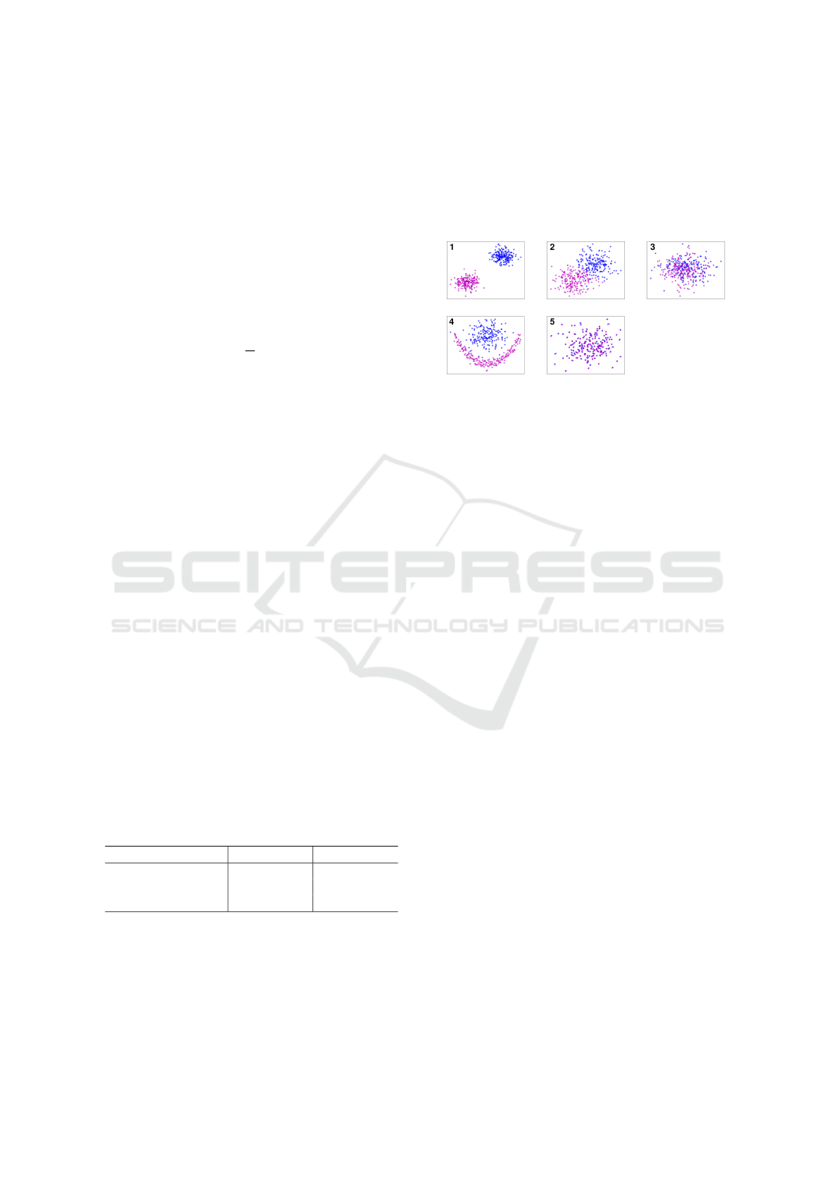
dataset. We have presented five major hypotheses in
Figure 8 to explain why the accuracy drops dramati-
cally on the UPMC-101 dataset. Assuming the source
dataset X
s
(blue) and the target dataset X
t
(magenta),
each sample in these figures belongs to one of these
datasets. Also, each dataset is represented using a dif-
ferent color.
Figure 8: Five major hypotheses for explaining the accuracy
drop on the UPMC-101 dataset. Samples with similar color
belong to the same dataset.
In the first plot, samples of the two datasets are
perfectly separable using a linear classifier. Samples
of X
s
partially cover the input space where there is not
any sample from X
t
in this part of the feature space.
Consequently, if we train the model on X
s
the model
is unlikely to generalize on samples from X
t
since this
part of the feature space is completely novel to the
model. In the second plot, the two regions slightly
overlap. In this scenario, the model might be able to
correctly classify some samples from X
t
. In the third
scenario, the two datasets occupy a common region in
the feature space. Nonetheless, there are some parts
in this region which are only covered by one of the
datasets. Therefore, the network may make mistake
in classifying samples belonging to these regions.
In the fourth plot, the two datasets form two dis-
tinct clusters that are non-linearly separable. This
may also cause the network to incorrectly classify
samples of X
t
. In the fifth plot, the two datasets are
aligned properly and distribution of samples in X
t
are
very similar to X
s
. It is worth mentioning that we can
define other hypotheses but, here, we only explained
these five hypotheses.
5.1 Domain Divergence
One way to estimate the divergence between the two
domains in the first and second scenarios is to train a
linear classifier to discriminate the samples of X
s
from
the samples of X
t
. Clearly, this is a binary classifica-
tion problem where samples coming from X
s
could be
labeled as “positive” or 1 and samples coming from X
t
could be labeled as “negative” or 0. Here, X
s
and X
t
include the feature vector extracted by the network. In
the case of the Inception V3, this is analogous to the
A Modified Self-training Method for Adapting Domains in the Task of Food Classification
149
output of the global average pooling layer which is
a 2048-dimensional vector. X
s
is created by entering
the samples from the Food-101 dataset to the network
and collecting their feature vectors. Likewise, X
t
is
created by entering the samples from the UPMC-101
dataset to the network and collecting their feature vec-
tors.
The classification accuracy in the first scenario
would be 100% and it would be less than 100% in the
second scenario depending on the amount of overlap.
The linear classifier in the remaining scenarios will
not be able to discriminate the two domains. Howe-
ver, a non-linear classifier is potentially able to discri-
minate the two domains in some of these scenarios.
We could design different networks with various
degrees of non-linearity and train them to discrimi-
nate X
s
and X
t
. Then, based on the accuracy of each
network we could infer the scenario that describes the
divergence between X
t
and X
s
. Instead of designing
different architectures for each of these situations, we
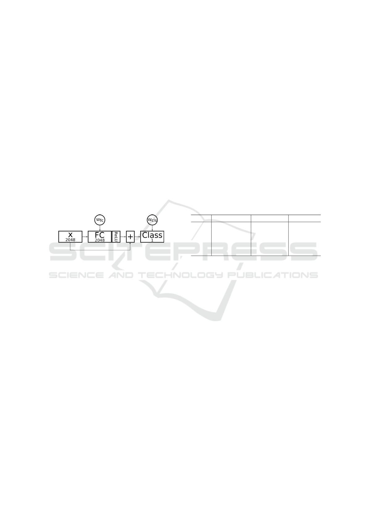
designed the network illustrated in 9.
Figure 9: Architecture of the domain classifier. The num-
ber in rectangles show the number of neurons in that layer.
In the case of input x, the number indicates the number of
elements of the input. Here, FC denote a fully connected
layer.
Formally, our network is defined as:
Θ(x) = relu(w
f c
· x) + x
p(x) = σ(w
cls
· Θ(x))
(11)
where w
f c
is the weight vector of the fully connected
layer and w
cls
is the weight vector of the classification
layer. We train the network by minimizing:
E = H(y
x
, p(x)) + γ||w
f c
||
2
+ λ||w
cls
||
2
. (12)
where y
x
is the binary label and H is the binary cross
entropy loss. The binary label y
x
is 1 for samples
coming from the Food-101 datasets and it is set to
0 for samples coming from the UPMC-101 dataset.
We regularize the classifier different from the non-
linear transformation layer. Specifically, if we are in-
terested in a classifier which acts similar to a linear
classifier, we set γ to a large number in order to en-
courage the weights of this layer (w
f c
) to be very
close to zero. When w
f c
is zero or very close to
zero, |relu(w
f c
· x)| = ε will become zero or close to
zero. In other words, the input of the classifier will be
Θ(x) = ε + x showing that the input enters the classi-
fier almost without any modification. In this case, the
whole network will be actually a linear classifier.
Conversely, by reducing the value of γ, we let the
network to learn nonlinear boundaries with a higher
degree of non-linearity. To be more specific, this will
cause the weight vector w
f c
to have non-zero ele-
ments. This will cause that relu(w
f c
· x) to have non-
zero elements. As the result, the input x will be modi-
fied non-linearly which will make the whole network
a non-linear classifier.
We collected X
s
and X
t
as we mentioned above af-
ter adapting the knowledge of the Inception V3 on the
Food-101 dataset. Then, we fixed λ to 1e− 5 and trai-
ned the network using different values for γ. Finally,
we trained the classifier to discriminate the training
set of the Food-101 dataset from the test set of the
UPMC-101 dataset. Table 2 shows the results.
Table 2: Classification accuracy of the domain classifier for
different values of γ trained to classify the training set of the
Food-101 and the test set of the UPMC-101 datasets.
γ Accuracy (%) Precision(%) Recall (%)
linear 69.06 67.35 74.01
1 71.94 69.98 76.83
0.1 88.19 87.01 89.80
0.01 96.50 96.19 96.82
0.001 99.99 1.00 99.99
Surprisingly, a linear classifier is able to discrimi-
nate 69.06% of the samples from these two datasets,
correctly. Then, we increased the non-linearity of the
network by reducing the value of γ. As the value of
γ reduces, the network becomes more flexible and it
is able to discriminate the two domains more accura-
tely. We observe that by setting γ to 0.01, the network
is able to differentiate 96.50% of Food-101 samples
from the UPMC-101 samples. In addition, by setting
γ to 0.001 the network is able to discriminate 99.99%
of Food-101 samples from the UPMC-101 samples
correctly. This analysis suggests that the second and
fourth hypotheses might be true on the Food101 and
UPMC-101 datasets. In other words, the two data-
sets have diverged and this is one of the reasons that
our network performs poorly when it is trained on the
Food-101 dataset and tested on the UPMC-101 data-
set.
5.2 Modified Self-training
Next, we utilized our modified self-training approach
for adapting the domain from the Food-101 to the
UPMC-101. We assume that labels of the UPMC-
101 dataset are not available during training. In other
words, we perform unsupervised domain adaptation.
VISAPP 2019 - 14th International Conference on Computer Vision Theory and Applications
150

We applied the domain classifier from the previous
section to discriminate the training and test sets of the
UPMC-101 dataset. Table 3 shows the results.
Table 3: Classification accuracy of the domain classifier for
different values of γ trained to classify the training set and
the test set of the UPMC-101 datasets.
γ Accuracy (%) Precision(%) Recall (%)
linear 54.39 54.35 54.90
1 54.83 54.80 55.21
0.1 55.44 55.31 56.68
0.01 55.64 55.48 57.11
0.001 83.00 81.76 84.96
0.0001 90.81 88.31 94.08
Compared to Table 2, we realize that the linear
classifier is only able to discriminate 54.39% of sam-
ples correctly which is 14.67% is less than the same
classifier in Table 2. Also, we notice that the accuracy
of the domain classifier is less than 56% when the va-
lue of γ is greater than or equal to 0.01. However, the
accuracy jumps considerably by setting γ to 0.001 or
lower. These results suggest that divergence between
the training and test sets of the UPMC-101 dataset is
potentially less than the divergence between the test
of the UPMC-101 dataset and the training set of the
Food-101 dataset.
From another perspective, if the network is trained
on the training set of the UPMC-101 dataset and tes-
ted on the test set of the UPMC-101 dataset, it is likely
to perform better than training the network using the
Food-101 dataset and assessing them on the UPMC-
101 dataset. In order to estimate what could be the lo-
wer bound of the error on the UPMC-101 dataset, we
adapted the knowledge of the network to the training
set of the UPMC-101 dataset. Table 4 compares our
results with the results obtained by the UPMC Team
1
.
As our analysis using the domain classifier sugge-
sted, training the network using the UPMC-101 data-
set provides more accurate results. Since the Food-
101 dataset is more diverged from the test set of
the UPMC-101 compared to the training set of the
UPMC-101, the classification accuracy after adapting
the domain (not knowledge) of the Food-101 to the
UPMC-101 might not be greater than 71.05% in the
best case scenario using single image validation. In
other words, denoting the classification accuracy of
our model on the UPMC-101 dataset by acc
upmc
, we
suppose that acc
upmc
is bounded within
58.61% ≤ acc
upmc
≤ 71.05% (13)
when it utilizes the Food-101 dataset for training and
the unlabeled training set of the UPMC-101 dataset
1
blog.heuritech.com
for adapting the domain of the model. Next, we ap-
plied our proposed self-training approach for adap-
ting the domain of the network to the UPMC-101 da-
taset. Specifically, we used our network trained on
the Food-101 dataset and used the training set of the
UPMC-101 dataset as the unlabeled target dataset.
Then, we performed domain adaptation and assessed
the results on the test set of the UPMC-101 dataset.
Table 4 shows the results.
According to the results, Tri-training increases
the classification accuracy to 60.81% and our modi-
fied self-training approach improves the results up to
62.66%. It is worth mentioning that our method is
faster to run and setting its hyperparameters is fairly
trivial. Also, we did not compare our method with ot-
hers methods because Tri-Training approach has sur-
passed the performance of other methods in literature
(Saito et al., 2017). Figure 10 and Figure 11 shows
the precision and recall before and after performing
self-training.
We notice that the mean precision, minimum pre-
cision, and the maximum precision have been impro-
ved after adapting the domain. The recall also shows
a similar behavior and mean recall, minimum recall,
and maximum recall have been improved using our
method. This is due to the fact that our method select
samples whose prediction uncertainty is low. We ana-
lyzed the network before and after adaptation using
the class activation mapping (CAM) technique (Zhou
et al., 2015). Figure 12 shows a few samples from the
UPMC dataset.
The first row in this figure shows the query image.
All images in this figure are incorrectly classified be-
fore adapting the domain and all of them are classified
correctly after applying our proposed method. The
second row is the CAM of actual class before adap-
ting the domain. The third row shows the CAM of the
predicted class before adapting the domain. The last
row illustrates the CAM of the predicted class after
adapting the domain. We observe that the CAM of
the network has been changed and moved after adap-
tation.
For example, the second column shows the image
of a “cannoli”. However, it is classified as “Peking
duck” before adaptation. After applying our propo-
sed self-training approach, the network shifts the at-
tention to another part of the image. After adapting
the attention, the network is able to predict the image
correctly.
A Modified Self-training Method for Adapting Domains in the Task of Food Classification
151
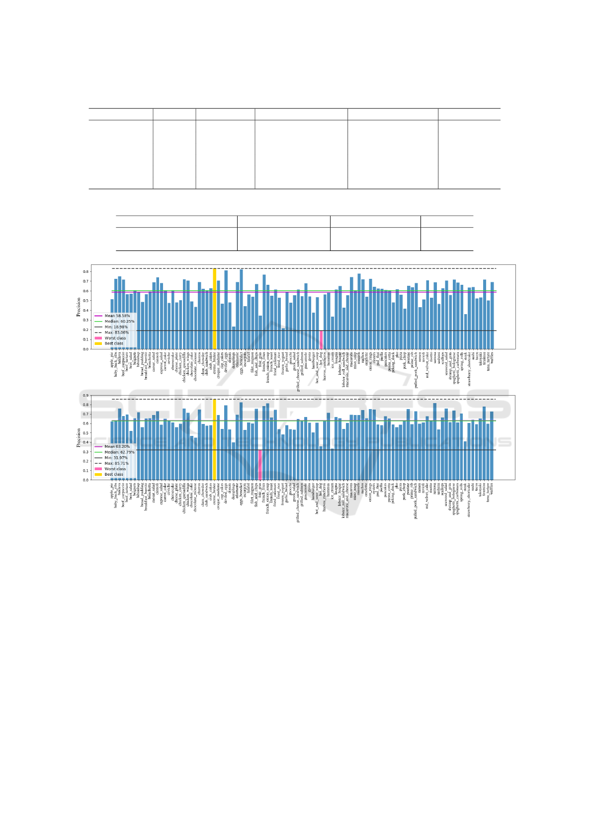
Table 4: Classification accuracy of the UPMC-101 dataset when the network is trained on different training sets.
Model Method Training set Accuracy Top-1 (%) Accuracy Top-5(%) evaluation
our KA Food-101 60.02 77.57 multi-crop
our KA Food-101 58.61 76.61 single image
our KA UPMC-101 73 87.29 multi-crop
our KA UPMC-101 71.05 86 single image
UPMC Team KA UPMC-101 66.83 NA NA
UPMC Team scratch UPMC-101 53.62 NA NA
Table 5: Classification accuracy on the UPMC-101 dataset after adapting the knowledge of the network.
Method Accuracy Top-1 (%) Accuracy Top-5(%) evaluation
Tri-training 60.81 77.86 single
Modified self-training (our) 62.66 78.81 single
Figure 10: Precision of the network on the UPMC dataset before (top) and after (bottom) applying our modified self-training
approach (best viewed electronically).
6 CONCLUSION
In this paper, we proposed a new method based on
self-training in which we assign pseudo-labels to tar-
get samples taking into account the uncertainty of pre-
diction rather than their probability scores. To es-
timate the uncertainty, we utilized multi-crop multi-
scale evaluation with flipping and computed the mu-
tual information of predictions.
Next, we applied our network trained on the Food-
101 dataset to the UPMC-101 dataset and showed that
the accuracy drops to 58.61%. We further analyzed
this behavior using a domain classifier. To be more
specific, we designed a domain classifier with adapta-
ble nonlinearity and trained it to discriminate samples
of the Food-101 dataset from the UPMC-101 dataset.
We showed that a linear classifier is able to classify
69.06% of these samples correctly. This suggests that
there is a divergence between the two datasets even
though their label spaces are identical. We applied
our proposed method as well as the tri-training met-
hod to this problem. Our experiments showed that the
proposed method is able to produce superior results.
VISAPP 2019 - 14th International Conference on Computer Vision Theory and Applications
152
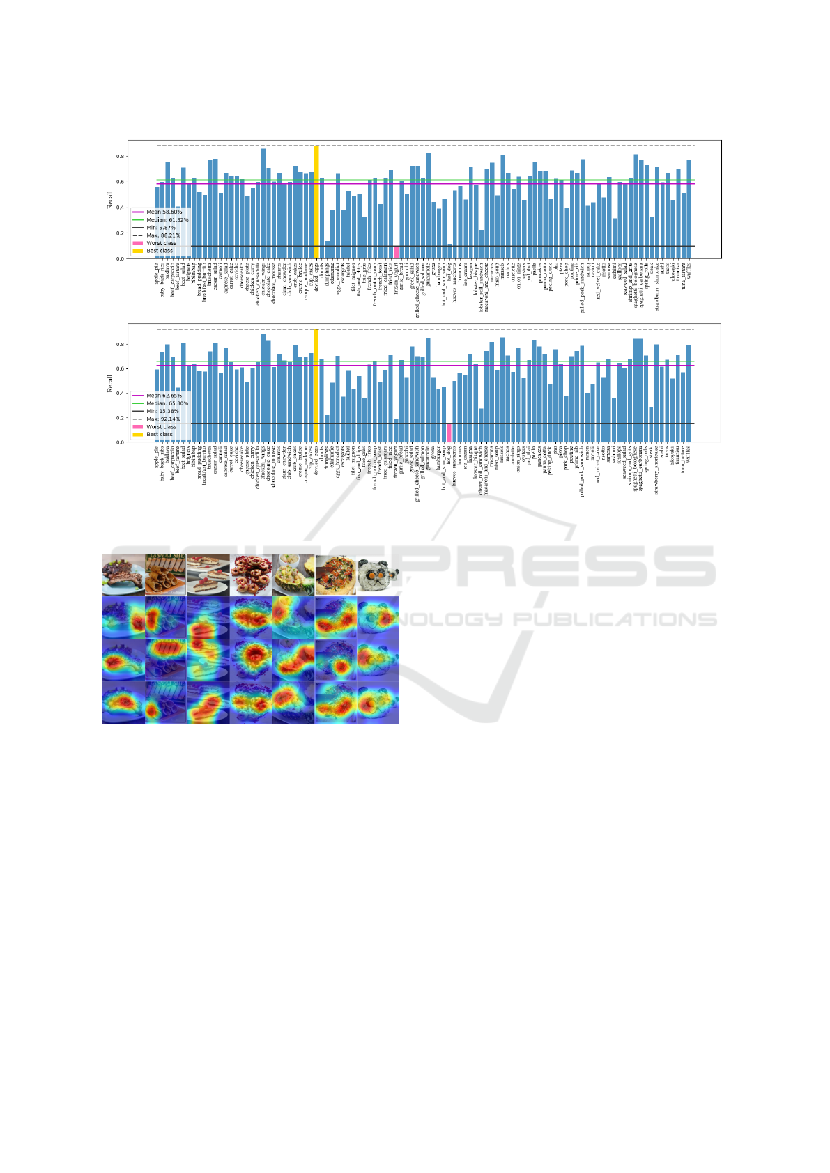
Figure 11: Recall of the network on the UPMC dataset before (top) and after (bottom) applying our modified self-training
approach (best viewed electronically).
Figure 12: Visualizing the network using CAM before and
after adaptation on a few samples from the UPMC dataset.
REFERENCES
Bossard, L., Guillaumin, M., and Van Gool, L. (2014).
Food-101 – Mining Discriminative Components with
Random Forests, pages 446–461. Springer Internatio-
nal Publishing.
Bousmalis, K., Silberman, N., Dohan, D., Erhan, D.,
and Krishnan, D. (2016a). Unsupervised Pixel-Level
Domain Adaptation with Generative Adversarial Net-
works.
Bousmalis, K., Trigeorgis, G., Silberman, N., Krishnan, D.,
and Erhan, D. (2016b). Domain Separation Networks.
(NIPS).
Creswell, A., White, T., Dumoulin, V., Arulkumaran, K.,
Sengupta, B., and Bharath, A. A. (2017). Generative
Adversarial Networks: An Overview. (April):1–14.
Csurka, G., Baradel, F., and Chidlovskii, B. (2017).
Discrepancy-based networks for unsupervised domain
adaptation : a comparative study. International Con-
ference on Computer Vision (ICCV), (1):2630–2636.
Fernando, B., Habrard, A., Sebban, M., and Tuytelaars, T.
(2013). Unsupervised visual domain adaptation using
subspace alignment. Proceedings of the IEEE Interna-
tional Conference on Computer Vision, pages 2960–
2967.
Ganin, Y. and Lempitsky, V. (2014). Unsupervised Domain
Adaptation by Backpropagation. (i).
Ganin, Y., Ustinova, E., Ajakan, H., Germain, P., Laro-
chelle, H., Laviolette, F., Marchand, M., and Lem-
pitsky, V. (2015). Domain-Adversarial Training of
Neural Networks. 17:1–35.
Ghifary, M., Kleijn, W. B., Zhang, M., Balduzzi, D., and
Li, W. (2016). Deep reconstruction-classification net-
works for unsupervised domain adaptation. Lecture
Notes in Computer Science (including subseries Lec-
ture Notes in Artificial Intelligence and Lecture Notes
in Bioinformatics), 9908 LNCS:597–613.
Goodfellow, I. J., Pouget-Abadie, J., Mirza, M., Xu, B.,
Warde-Farley, D., Ozair, S., Courville, A., and Ben-
gio, Y. (2014). Generative Adversarial Networks. pa-
ges 1–9.
Haeusser, P., Frerix, T., Mordvintsev, A., and Cremers, D.
(2017). Associative Domain Adaptation.
Hoffman, J., Tzeng, E., Park, T., Zhu, J.-Y., Isola, P., Sa-
enko, K., Efros, A. A., and Darrell, T. (2017). Cy-
A Modified Self-training Method for Adapting Domains in the Task of Food Classification
153

CADA: Cycle-Consistent Adversarial Domain Adap-
tation. pages 1–12.
Liu, M.-Y. and Tuzel, O. (2016). Coupled Generative Ad-
versarial Networks. (NIPS).
Long, M., Cao, Y., Wang, J., and Jordan, M. I. (2015). Lear-
ning Transferable Features with Deep Adaptation Net-
works. 37.
Long, M., Zhu, H., Wang, J., and Jordan, M. I.
(2016). Unsupervised Domain Adaptation with Re-
sidual Transfer Networks. (Nips).
Morerio, P., Cavazza, J., and Murino, V. (2017). Minimal-
Entropy Correlation Alignment for Unsupervised
Deep Domain Adaptation. (2011):1–14.
Ruder, S. and Plank, B. (2018). Strong baselines for neural
semi-supervised learning under domain shift. CoRR,
abs/1804.09530.
Saito, K., Ushiku, Y., and Harada, T. (2017). Asymmetric
Tri-training for Unsupervised Domain Adaptation.
Shaham, U., Stanton, K. P., Zhao, J., Li, H., Raddassi, K.,
Montgomery, R., and Kluger, Y. (2016). Removal of
Batch Effects using Distribution-Matching Residual
Networks.
Sun, B., Feng, J., and Saenko, K. (2015). Return of Frustra-
tingly Easy Domain Adaptation. (Figure 1).
Szegedy, C., Vanhoucke, V., Ioffe, S., Shlens, J., and Wojna,
Z. (2016). Rethinking the inception architecture for
computer vision. In IEEE Conference on Computer
Vision and Pattern Recognition, (CVPR), pages 2818–
2826.
Torralba, A. and Efros, A. A. (2011). Unbiased Look at
Dataset Bias.
Tzeng, E., Hoffman, J., Darrell, T., Saenko, K., and Lowell,
U. (2015). Simultaneous Deep Transfer Across Dom-
ains and Tasks. International Conference on Compu-
ter Vision (ICCV).
Tzeng, E., Hoffman, J., Saenko, K., and Darrell, T. (2017).
Adversarial Discriminative Domain Adaptation.
Tzeng, E., Hoffman, J., Zhang, N., Saenko, K., and Darrell,
T. (2014). Deep Domain Confusion: Maximizing for
Domain Invariance.
Wang, X., Kumar, D., Thome, N., Cord, M., and Precioso,
F. (2015). Recipe recognition with large multimodal
food dataset. 2015 IEEE International Conference
on Multimedia and Expo Workshops, ICMEW 2015,
(1):2–7.
Wang, Y., Li, W., Dai, D., and Van Gool, L. (2017). Deep
Domain Adaptation by Geodesic Distance Minimiza-
tion.
Zhou, B., Khosla, A., Lapedriza,
`
A., Oliva, A., and
Torralba, A. (2015). Learning deep features for dis-
criminative localization. CoRR, abs/1512.04150.
VISAPP 2019 - 14th International Conference on Computer Vision Theory and Applications
154
