Improving Transfer Learning Performance: An Application in the

Classiﬁcation of Remote Sensing Data

Gabriel Lins Tenorio, Cristian E. Munoz Villalobos, Leonardo A. Forero Mendoza,

Eduardo Costa da Silva and Wouter Caarls

Electrical Engineering Department (DEE), Catholic University of Rio de Janeiro - PUC-Rio, Rio de Janeiro, Brazil

Keywords:

Deep Learning, Convolutional Neural Networks, Transfer Learning, Fine Tuning, Data Augmentation,

Distributed Learning, Cross Validation, Remote Sensing, Vegetation Monitoring.

Abstract:

The present paper aims to train and analyze Convolutional Neural Networks (CNN or ConvNets) capable of

classifying plant species of a certain region for applications in an environmental monitoring system. In order

to achieve this for a limited training dataset, the samples were expanded with the use of a data generator

algorithm. Next, transfer learning and ﬁne tuning methods were applied with pre-trained networks. With the

purpose of choosing the best layers to be transferred, a statistical dispersion method was proposed. Through

a distributed training method, the training speed and performance for the CNN in CPUs was improved. After

tuning the parameters of interest in the resulting network by the cross-validation method, the learning capacity

of the network was veriﬁed. The obtained results indicate an accuracy of about 97%, which was acquired

transferring the pre-trained ﬁrst seven convolutional layers of the VGG-16 network to a new sixteen-layer

convolutional network in which the ﬁnal training was performed. This represents an improvement over the

state of the art, which had an accuracy of 91% on the same dataset.

1 INTRODUCTION

Vegetation monitoring can be done by farmers to dis-

tinguish plants, check planting failures and verify

vegetation health and growth. The visual distinction

of plants is useful to identify unwanted plants (weed)

that deteriorate the health of several species of vege-

tation (Aitkenhead et al., 2003). Such monitoring can

be difﬁcult when the plantation area is large or when

it is fenced by plants. A possible solution is the use

of a remote sensing monitoring system using images

from satellites.

Some satellites use multispectral sensors which

provide images of the visible and invisible spectrum.

The reﬂectance of a plant at a certain wavelength de-

pends on the ﬂux of radiation that reaches it and on

the ﬂux that is reﬂected. This second variable is con-

ventionally observed in the intensity levels of a plant

image in the invisible spectrum of light, as the near

infrared spectrum is reﬂected by the cell structure of

plants with high magnitude, varying between differ-

ent plants (Horler et al., 1983).

The dataset analyzed in this work was obtained

through photo captures taken by the RapidEye Ger-

man satellite system, which provides multispectral

data. The dataset contains images from different areas

containing four classes of plants: agriculture, arboreal

vegetation, herbaceous vegetation and shrubby vege-

tation, present in the Serra do Cipo region in the cen-

tral area of southern Brazil (Nogueira et al., 2016).

For this task, the green, red and near-infrared bands

are appropriate for distinguishing the classes of inter-

est (Nogueira et al., 2016). Each image taken by the

satellite contains various plant species, making it nec-

essary to consult specialists for separating and classi-

fying them. Thus, a class distribution of the dataset

with 1311 multispectral scenes is obtained.

The recognition of the specie’s patterns was one of

the main difﬁculties discussed by the original authors

regarding the interpretation of the images contained

in the dataset, given their complex intraclass vari-

ance and interclass similarity (Nogueira et al., 2016).

These issues make the sample preparation and sep-

aration into groups costly and limited. As a conse-

quence, there are complex and unbalanced samples

so that classiﬁcation algorithms such as usual ANN

(Artiﬁcial Neural Networks), SVM (Support Vector

Machine) and decision-tree provide unsatisfactory re-

sults for this task. However, literature shows that deep

learning approaches (i.e. Convolutional Neural Net-

174

Tenorio, G., Villalobos, C., Mendoza, L., Costa da Silva, E. and Caarls, W.

Improving Transfer Learning Performance: An Application in the Classiﬁcation of Remote Sensing Data.

DOI: 10.5220/0007372201740183

In Proceedings of the 11th International Conference on Agents and Artiﬁcial Intelligence (ICAART 2019), pages 174-183

ISBN: 978-989-758-350-6

work - CNN) and other methods (i.e. data augmenta-

tion, transfer learning and ﬁne tuning), have a much

better performance in these cases, because they allow

to model and train a classiﬁer, (e.g. distinguishing

vegetation) using images as inputs, even with scarcity

and complexity of data (Gu et al., 2018). In this paper,

we begin by describing CNN deep learning models

and the motivation to use transfer learning and ﬁne-

tuning methods. Then, the solution strategy for the

classiﬁcation task is presented along with approaches

called data augmentation and cross-validation, to deal

with few and unbalanced data. We also show in the-

ory and experimentally how hyperparameters for the

model, the methods and the approaches described af-

fect the training performance. In order to train the

model with different layer topologies, a statistical dis-

persion method is proposed to evaluate each convo-

lutive layer of the model and help to choose which

layers are the best to be transferred to the ﬁne tune

model.

To increase considerably the training speed for

the CNN in a CPU, parallelism operators and a dis-

tributed learning method were used, which simulates

larger minibatches by dividing the data through work-

ers. Our experiments are then compared to baselines

and state of the art approaches, indicating superior re-

sults.

2 THEORETICAL FRAMEWORK

The convolutional neural network is a type of deep

learning architecture that has recently stood out in the

image recognition ﬁeld achieving a very high accu-

racy (Gu et al., 2018). The inputs of a CNN classiﬁer

are given by digital images, in the form of tensors,

that are brought to feature extractors. Each extrac-

tor performs operations, through ﬁlters, in parallel to

extract features from the images starting from more

generic, low-level features and culminating in higher

level features that are more speciﬁc to the dataset. A

second Neural Network is conventionally placed after

the last convolutional layer to operate as a classiﬁer.

As the complexity of the images increases, there

is a need to change CNN hyperparameters. However,

as the number of convolutional layers, the ﬁlter size

Table 1: Original Species Samples.

Species #Samples Proportion (%)

AGR 47 3.58

FOR 962 73.37

HRB 191 14.57

SHR 111 8.46

Total 1311 100

and number of CNN ﬁlters are increased, the com-

putational cost increases signiﬁcantly (He and Sun,

2015). This effect adds difﬁculties in experimental

research involving real applications, such as those re-

quiring rapid scenario changes

1, 2

being necessary to

explore the architecture’s parallelism capacity.

An approach called Transfer Learning (TL) may

decrease the number of required operations allow-

ing the transfer of learning, acquired in one prob-

lem, to another problem with similar characteris-

tics. What makes TL more effective is the pos-

sibility of using pre-trained networks such as VG-

GNet (Simonyan et al., 2013), GoogleNet (Szegedy

et al., 2015), ResNet (He et al., 2016) and AlexNet

(Krizhevsky et al., 2012), which stood out in the chal-

lenges of the Large Scale Visual Recognition Chal-

lenge (ILSVRC - ImageNet) for object detection and

image recognition (Russakovsky et al., 2015).

In models that require more speciﬁc classiﬁcation,

as in the scope of this paper, there is a need for Fine-

Tuning (FT) the model, freezing some layers of the

pre-trained networks and constructing convolutional

layers on top of them.

3 SOLUTION STRATEGY

3.1 Preparation of Data and Data

Augmentation

The dataset used for the network training

was found

in the paper by (K. Nogueira et al. 2016) which

also uses the artiﬁce of convolutional networks for

the classiﬁcation of four distinct vegetative species,

as shown in Fig. 1. The resolution of each image is

64 x 64 pixels.

The dataset has unbalanced and scarce samples

making it difﬁcult to develop the classiﬁcation model.

Table 1 shows the distribution of samples between

classes.

Some approaches can be used to train neural net-

works with unbalanced data avoiding the problem of

limited generalization, such as penalizing with higher

weights the errors of classiﬁcation of classes with less

Drive.ai, ”Building the Brain of Self-Driving Vehi-

cles”, 2018. Available: https://www.drive.ai/ [January 29,

2018].

Descartes Labs, ”A data reﬁnery, built to un-

derstand our planet”, 2017. Available: https://

www.descarteslabs.com/ [August 15, 2017]

The dataset is available for download at http://

www.patreo.dcc.ufmg.br/2017/11/12/brazilian-cerrado-

savanna-scenes-dataset/ [December 6, 2018].

Improving Transfer Learning Performance: An Application in the Classiﬁcation of Remote Sensing Data

175

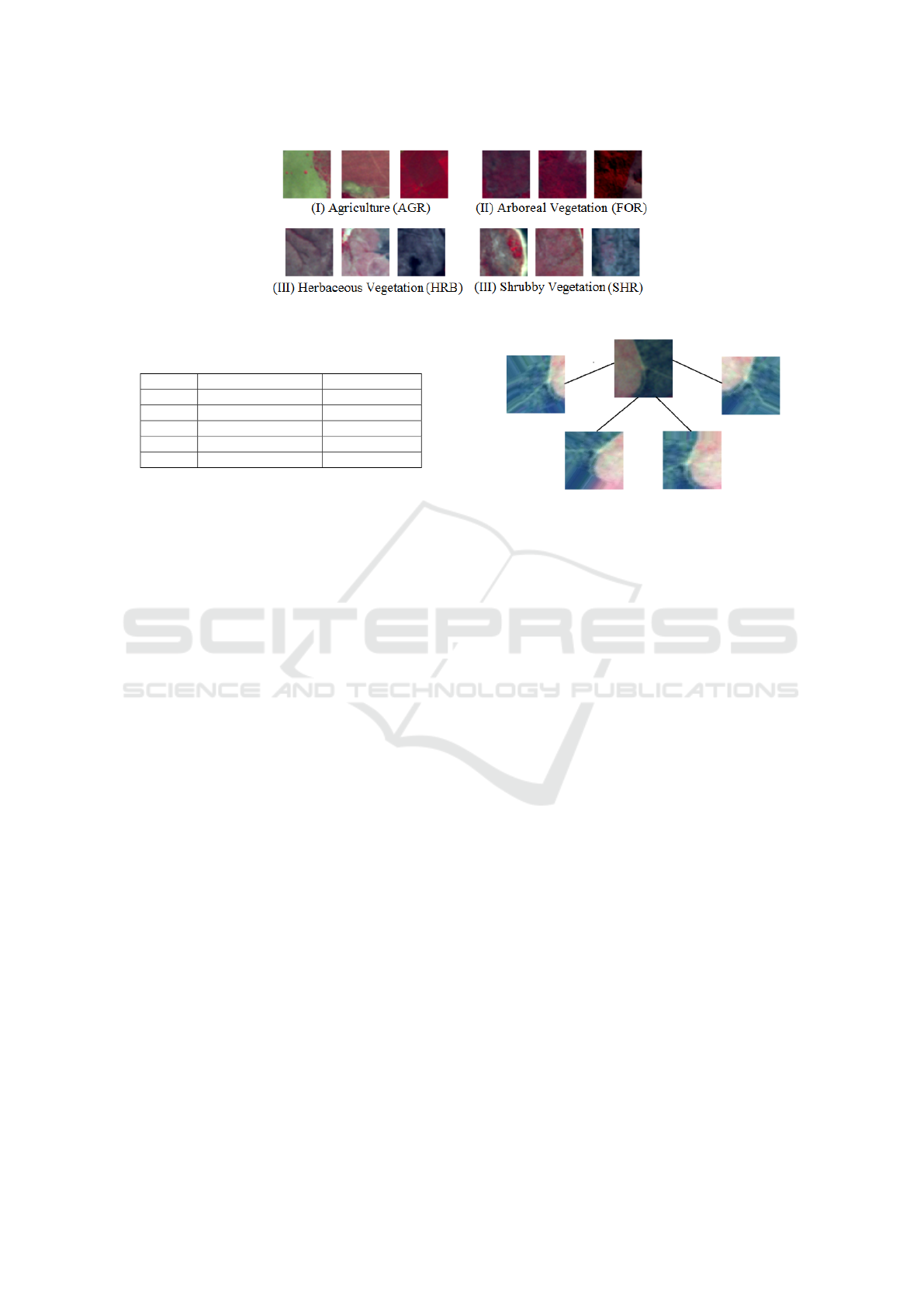
Figure 1: Group of four classes: AGR, FOR, HRB and SHR.

Table 2: Balanced classes samples generated using Keras

ImageDataGenerator in each new training.

Species # Training Samples # Test Samples

AGR 1770 540

FOR 1770 540

HRB 1770 540

SHR 1770 540

Total 7080 2160

samples. Another approach makes it possible to in-

crease the amount of data of each class proportion-

ally, thus balancing the data. In this article, the sec-

ond approach was chosen to solve the problem of

data scarcity. Another advantage of the data increase

in a neural network is that it acts as a regularizer,

making the model more robust, preventing overﬁtting

(Cires¸an et al., 2010) and improving the performance

of unbalanced models (Chawla et al., 2002).

Through the ImageDataGenerator from the

python deep learning library keras, it becomes pos-

sible to generate new images from the dataset with

random transformations applied to an image. We

used the following transformations: width and height

displacement, shear range, zoom, horizontal rotation,

and brightness adjustment. Figure 2 illustrates four

examples of random transformations in a single im-

age. Before increasing the data, the original dataset is

divided into training and test sets, respectively, 75%

and 25% of the samples. The same sets are used in all

experiments. Then, in each new training, the original

training set is balanced, proportionally to each class,

through data augmentation. After each training, the

test set is also expanded proportionally. Table 2 illus-

trates the increase of data using the image generator

for the training and test sets.

3.2 Pre-trained Network and Transfer

Learning

The training of many-layered convolutional networks,

based on the random initialization of weights, re-

quires a high computational cost due to the amount

of parallel operations that feature extractor ﬁlters per-

form. Using pre-trained networks it is possible to

minimize this cost initializing pre-trained weights and

Figure 2: Examples of transformations performed by the

Keras ImageDataGenerator in a single image.

bias thereby reaching the convergence of the model

much earlier. There are several models of pretrained

networks such as VGGNet, GoogleNet, ResNet and

AlexNet. In this paper, the VGG-16 network was cho-

sen, because it stands out for its uniform and effective

architecture for applications involving image classiﬁ-

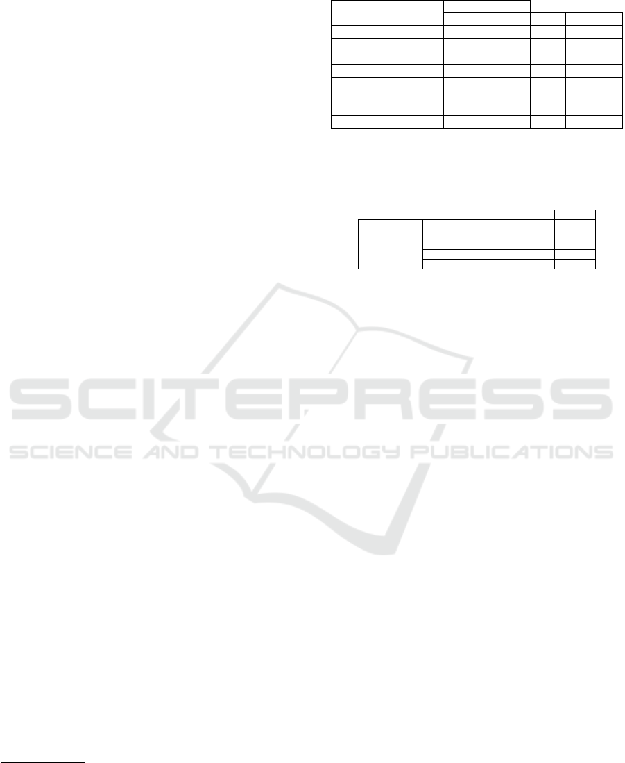
cation. The sixteen layers of the VGG-16 network use

only 3 x 3 convolution order and 2 x 2 order pooling.

Convolution is an image ﬁltering process that aims

to detect patterns creating feature maps. The pooling

process reduces the spatial size of the features discov-

ered by the convolution layers. Fig. 3 shows the ar-

chitecture of the VGG-16 networks (Gu et al., 2018).

The VGG-16 network is pre-trained using the Im-

ageNet database. This database has about fourteen

million high quality natural images with more than a

thousand labeled categories, that is, classes with their

proper titles.

Transfer learning is a technique that uses pre-

trained networks which take the generic features of

images, such as color blobs, edges and corners in the

ﬁrst layers. At each subsequent layer, the character-

istics taken from the images become more and more

speciﬁc with the training datasets which can be ob-

tained, for example, from the imagenet database. Af-

ter the training step, the classiﬁcation layers of the

pre-trained network (layers 14 to 16) are removed,

keeping the previous ones frozen (ﬁxed). The images

of the target dataset are executed in this truncated net-

work in order to produce bottleneck features. These

features are used to train a new classiﬁer and obtain

the prediction of the target dataset classes.

ICAART 2019 - 11th International Conference on Agents and Artiﬁcial Intelligence

176

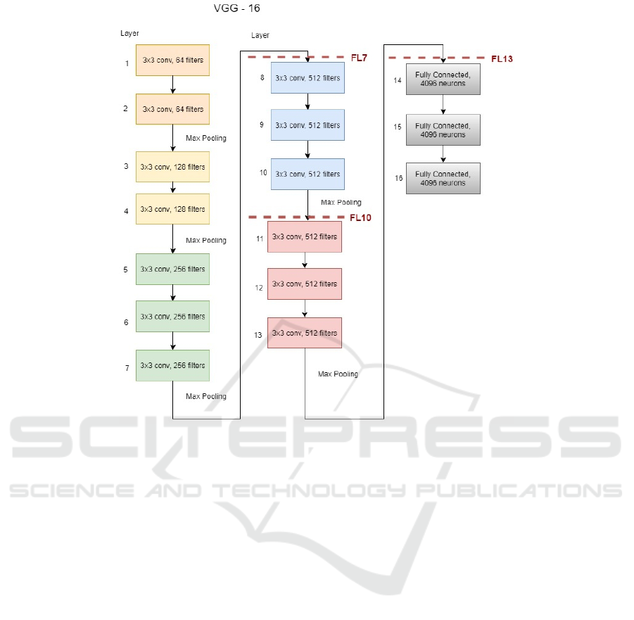
Figure 3: VGG-16 networks architecture. The codes next to the dotted lines indicate the frozen layers in the experiments.

Our target dataset has few samples, besides being

very different from the pre-trained network’s dataset,

so truncating the last layer of that network may not

be enough to obtain a satisfactory accuracy. This

is because features taken from the layers closest to

the output are not useful for the classiﬁcation of the

model. One solution to this problem is ﬁne tun-

ing which allows the lower Y layers of the transfer-

learning network to be frozen extracting characteris-

tics from these layers and after the last layer, new con-

volution and classiﬁcation layers can be added. A new

training of the resulting network can be performed,

taking into account that the weights and bias of the

Y layers are ﬁxed. Freezing more layers results in a

network with lower accuracy in exchange for a train-

ing that requires less computational complexity, as the

training of a network with less convolutional layers

demands less complexity to be calculated. In addi-

tion to the freezing of layers, the ﬁne tuning method

is also related to the tuning of the hyperparameters of

the resulting network.

3.3 Cross-validation

In order to evaluate the learning algorithm and how it

responds to the data augmentation, a cross-validation

metric is used. The cross validation divides the sam-

ples of the increased training set into different train-

ing and validation samples by making combinations

between them. A speciﬁc case of cross-validation is

the k-Fold cross-validation method, which divides the

samples into k

subsets at random and without repeti-

tion, using all the data in that division. The convolu-

tional neural network model is trained k

times, where

in each training a single subset is selected for the

test and k

− 1 subsets for the training. The method

is commonly used in Machine Learning applications

with 10 folds (k

= 10) aiming at adjusting the gener-

alization of the algorithm (Refaeilzadeh et al., 2009).

In order to obtain a resulting accuracy, the average of

the k

trainings is calculated.

3.4 CNN Layer Statistical Analysis

The output of each CNN layer is a feature map. In-

terpreting the feature maps in-between the layers may

show how well and in which layers the model is learn-

ing the speciﬁc features of each class. However, they

are not trivially interpretable and consequently it is

difﬁcult to choose the best layers to be frozen.

Some algorithms for dimensionally reduction (i.e.

PCA or t-SNE) can lead us to check whether, in a

Improving Transfer Learning Performance: An Application in the Classiﬁcation of Remote Sensing Data

177

certain convolutional layer, the features of each class

was separated by reducing the dimensionally to two

features and drawing a scatter plot (Jolliffe, 2011;

Maaten and Hinton, 2008). However, in some cases,

it is difﬁcult to verify whether the CNN has been able

to separate the features or whether the algorithm has

been able to reduce the dimension correctly. Another

algorithm that can be used to interpret the features

maps in CNNs is called DeepResolve (Liu and Gif-

ford, 2017). It is based on a gradient-ascent method

and does not require inputs by calculating a class-

speciﬁc optimal ’image’ H for each class in each layer

(Simonyan et al., 2013). This method’s output pro-

vides helpful information to analyze and decide which

layers are important to be frozen.

We propose a simpler statistical analysis of each

convolutional layer by calculating the mean of the

between-class standard deviation vector, for each

layer, which is calculated between the mean feature

maps of all classes.

Each three-dimensional feature map matrix is re-

shaped into a single dimension of vector (feature vec-

tor). The standard deviation vector previously men-

tioned is given by (1):

∑

n=1



−



N − 1

(1)

Where

is the mean feature vector between all

the images from class n in convolutional layer m and

is the mean vector between the classes in a given

layer. Those terms can be calculated by (2):

∑

j=1

∑

n=1

(2)

Where

denotes the feature vector from class n

in a layer m of image j and J

is the number of im-

ages in a given class n. Replacing the equations (2) in

equation (1), we calculate the vector

and the scalar

mean M

(3).

(3)

The number of classes is four (N = 4) and the

maximum number of convolutional layers is thirteen

(m = [1, 2,..13]). It is expected that the mean of the

inter-class standard deviation in each layer (M

) in-

creases because higher layers extract more speciﬁc

features, which should therefore exhibit larger inter-

class variance. This variable could tell which is the

appropriate convolutional layer that should be frozen

and then perform a new training. For example, if the

variable decreases considerably in a given layer, this

means that the features are getting worse on the new

domain (they are too speciﬁc to the original domain),

and therefore it is not useful to freeze that layer.

3.5 Distributed Training using Large

Minibatches

In order to take advantage of the computational power

of a multi-core CPU and increase the training speed

effectively, a distributed training method was used.

The method proposed by (Goyal et al., 2018) sim-

ulates large minibatches of size kn by dividing the

batches of the dataset through k workers not compro-

mising, until a certain point, the model’s accuracy. In

order to maintain the same behavior as a regular mini-

batch of size n, the method uses a linear scaling rule

which consists in multiplying the learning rate (η) by

the number of workers (k). An assumption is made

for this rule to take effect as shown in equation 4.

∇l(x, w

t+ j

) ≈ ∇l(x, w

), where j < k (4)

The ﬁrst term ∇l(x,w

t+ j

) represents the gradient

of the loss function for a sample x and weights w

t+ j

the training iteration t + j. The gradient is used in the

minibatch Stochastic Gradient Descent (SGD) with a

learning rate η and small minibatch of size n (Goyal

et al., 2018). For the large minibatch, the loss is only

calculated using the second term ∇l(x, w

). With the

previous assumption and setting a new learning rate

(

η) proportional to the number workers (

η = kη), the

SGD updates from small and large minibatch is sim-

ilar (Goyal et al., 2018). As an effect, increasing

the batch size should not substantially affect the loss

function optimization. As described by the authors,

the assumption is not true at the beginning of the train-

ing when the weights are changing quickly. To solve

this problem a gradual warmup is used, starting the

training from a base learning rate η and increasing

this value constantly until it reaches the learning rate

η proportional to k after 5 epochs (Goyal et al., 2018).

Additionally, the learning rate is divided by 10 at the

, 60

and 80

epochs, similar to (He et al., 2016).

3.6 Experiments

The experiments performed in this work were carried

out on two Intel



Xeon



Platinum 8160 CPUs with

24 cores each (96 threads in total) and 192GB of RAM

that made possible the application of the distributed

training and considerably increase the training speed.

The implemented model was simulated in the

Keras framework with Intel



Tensorﬂow backend

that allows the use of dataﬂow programming. Also,

Intel



MKL-DNN that accelerates the Deep Learning

framework on Intel



processors (allowing the use of

ICAART 2019 - 11th International Conference on Agents and Artiﬁcial Intelligence

178

Load Balance System Optimization

(LBSO) param-

eters) and the open source framework Horovod (as a

base of the distributed training) were used.

The experiments used transfer learning freezing Y

layers, denoted ”FL-Y”, and ﬁne tuning. Freezing of

the layers below 13 (FL-13), 10 (FL-10) and 7 (FL-7)

were performed as depicted in Fig. 3. It is relevant

to notice that all the convolutional layers in the FL-13

experiment are frozen which means that ﬁne tuning

method has no effect. For all experiments, the softmax

function was used in the output layer composed of

four neurons, which provides the degree of certainty

of an input image in relation to each of the four spec-

iﬁed classes. The class that contains the highest value

is chosen to represent the input image.

The impacts of variations of the hyperparameters

of interest, within predeﬁned ranges of values, on

the training time and resulting accuracy of the model

were analyzed in all experiments. These analyses

considered variations in parameters such as dropout,

number of epochs and base learning rate. Also, the

number of workers (k) and LBSO parameters such

as intra-operation parallelism (maximum number of

threads to run an operator) and inter-operation par-

allelism (maximum number of operators that can be

executed in parallel) were evaluated for the model’s

accuracy. Other parameters such as pooling size

and convolution ﬁlter size were kept ﬁxed in order

to avoid incompatibility with the architecture of the

pre-trained networks. For k-fold cross-validation the

value of k

= 10 was used, which results in better per-

formance in comparison to lower values of k

. The

SGD optimization algorithm was used for the all the

training experiments.

Table 3 presents the range of values in which the

hyperparameters of interest were evaluated and the

optimal values obtained experimentally.

The three experiments that provided the best re-

sults from the hyparameters adjustments and freezing

of the layers below 13 (FL − 13), 10 (FL − 10) and 7

(FL −7) were selected. As discussed previously, each

convolutional layer of the pre-trained network that is

not frozen (learning not transferred) must be added in

the ﬁne-tuning network. The three best experiments

and their topologies are shown in Table 4.

Boosting Deep Learning Training & Inference Per-

formance on Intel



Xeon



and Intel



Xeon Phi

Processors, 2018. Available: https://software.intel.com/en-

us/articles/boosting-deep-learning-training-inference-

performance-on-xeon-and-xeon-phi [November 5, 2018]

Table 3: Variation of hyperparameters of Interest (keeping

the batch size ﬁxed n = 32).

Parameter Range of Values

Min Max Optimal*

Dropout 0% 70% 50%

# Epochs 35 650 100

Base LR (η) 10

−5

−3

−5

# Workers (k) 1 12 5

Intra-op 2 48 19

Inter-op 0 4 2

Simul. Batch Size (kn) 32 384 160

Frozen Layers 7 13 7

*The optimal value is the best estimate found for the

parameter of interest

Table 4: Topologies of the FL − 13, FL − 10 and FL − 17

experiments.

FL-13 FL-10 FL-7

Convolutional Layers - 3 6

Filters - 128x3 512x6

Classiﬁcation Layers 2 1 2

Neurons 512-256 512 512-256

Dropout (%) 0-0 0.3 0.5-0

4 RESULTS AND DISCUSSIONS

In order to evaluate the performance of the model with

the different analyzed topologies, the three best ex-

periment conﬁgurations of each topology were com-

pared. Additionally, the full training experiment was

done. Each experiment was performed ten times,

calculating the uncertainty of the results and obtain-

ing more precise accuracy values. Table 5 indicates

the total simulation time of the training performed,

through 10-fold cross-validation, and the resulting ac-

curacy of each experiment. It is important to note that

in the original dataset, the proportion of the class with

more samples is 73.37%. Considering this observa-

tion, it is considered that values of weighted accu-

racy around 73% are unsatisfactory, because the clas-

siﬁer should be better than chance. To obtain results

that are comparable to the original paper, the overall

test accuracy of the experiments was also weighted

by each class proportion. At each fold of the k-Fold

cross-validation method, the model was saved to ob-

tain the class prediction and the normalized confusion

matrix on the augmented test set. The diagonal ele-

ments of this matrix show the normalized true posi-

tive predictions of each class which are then weighted

by each class proportion and added. This procedure

is repeated k

times and after that the overall test ac-

curacy was calculated. Table 6 shows the confusion

matrices of experiments FL-13, FL-10 and FL-7.

In order to evaluate the training time of the exper-

iment that demands most computational power (FL-

7) varying some hyperparameters for the distributed

learning (intra-op and k) and keeping the other op-

Improving Transfer Learning Performance: An Application in the Classiﬁcation of Remote Sensing Data

179

Table 5: Results FL − 13, FL − 10, FL − 7 and FL − 0.

Experiment Training Overall Test Overall Test

Time* Accuracy Accuracy

(Weighted)

FL − 13 15 min → 4 min 45.1 ± 1.9 % 79.43 ± 1.3 %

FL − 10 50 min → 12 min 81.8 ±1.4 % 76.7 ± 1.2 %

FL − 7 183 min → 37 min 97.3 ± 0.9 % 97.1 ± 1.0 %

FL − 0 567 min 55.7 ± 2.1 % 77.6 ±1.6 %

*The values indicates the decrease (→) of the training time

when using the Intel MKL-DNN as opposed to default

TensorFlow

timal values ﬁxed (as show in Table 3), the Table 7

was generated. For all the variations expressed, the

model’s loss function presents similar behavior and

ﬁnal values.

It is noted from the results presented in Tables 5

and 6 that the experiment FL-13 has high uncertainty,

regarding the achieved accuracy values and it is also

unreliable because the most predictions were just in a

single class. As noted earlier, the pre-trained network

learned from different datasets that are distinct when

compared to the dataset employed in this paper. Con-

sequently, only the lower-level features are useful for

classifying the speciﬁc vegetative species of interest

accurately.

Increasing the number of workers and intra-op, as

shown in Table 7, decreases the training time consid-

erably, but at certain point (k > 8) the model’s per-

formance decreases. Also, a proportionally low value

for intra-op in relation to k increases the training time

and, as a limitation, the multiplication of (k · Intra-op)

should be less than or equal to the number of total

threads (k · Intra-op ≤ 96). The best trade-off be-

tween performance and training time was obtained

when balancing intra-op and k values as shown in the

highlighted column in Table 7.

As discussed and described previously, it is also

possible to use a statistical method to ﬁnd the most

suitable layer to be frozen and train the deep learn-

ing model. Figure 4 shows a chart that contains the

mean of the inter-class standard deviation in each

layer (M

) for each experiment.

Looking at the lightest bars, it can be seen that

after the 9

convolutional layer the M

value re-

mains low, which conﬁrms that the model can’t ﬁnd

useful features that distinguish the classes. So, we

may choose to freeze all layers that are part of the 9

layer’s max-pooling block and below, leading to the

FL − 10 model.

Alternatively, observing that M

has a maximum

at the 6

layer, it is logical to freeze until there.

Again, ﬁxing the boundary to the max pooling block

leads to the FL − 7 model.

The FL −10 and FL−7 experiments provided su-

perior results compared to the FL − 13 experiment

that does not use ﬁne tuning. The expressive gain of

accuracy of the FL − 7 and reliability (the true class

prediction is more distributed through the classes) of

the experiment FL-10 are due to the ability of the con-

volutional networks, added in these experiments, to

learn the more speciﬁc features of the dataset used,

which was expected for these conﬁgurations. In rela-

tion to the training time, it can be seen that it tripled

with the addition of three convolution layers (FL −13

experiment to FL − 10) and tripled again by doubling

the convolution layers (FL − 10 to FL − 7). This

proves the expectation of computational complexity

attributed to training a network with more convolu-

tional layers.

The superior results can also be observed when

looking at the mean interclass standard deviations in

Figure 4. Both FL − 10 (dark grey bars) and FL −

7 (black bars) show higher deviations for the deeper

layers, but only FL − 7 maintains the upward trend of

separability.

It is important to note that, for the target dataset,

freezing less and less layers results in better results,

but in addition to the computational cost, the chances

of obtaining poor results are even greater with data

augmentation. This is due to, with this decrease, the

architecture is increasingly approaching the full train-

ing model (i.e., starting from scratch) having a much

larger number of parameters to be trained and possi-

bly overﬁtting the model during the training (Gu et al.,

2018). In order to conﬁrm this statement, the exper-

iment FL − 0 (training from scratch) was made and

the results are shown in table 5. For this experiment,

in the training phase, the model’s training and valida-

tion accuracies presented very high values, but in the

testing phase the overall test accuracy value was very

low, which indicates an overﬁtting of the data.

The baseline accuracies for this dataset predic-

tion proposed by the original authors were less than

82.5%, using different techniques as BIC (Stehling

et al., 2002), CCV (Pass et al., 1997), GCH (Swain

and Ballard, 1991) and UNSER (Unser, 1986) as seen

in Table 8.

The best accuracy obtained by the authors of the

article used as inspiration was 90.5 ± 1.8%. In the

mentioned paper, the AlexNet pre-trained network

architecture with ﬁne tuning and layer freezing was

used, but without data augmentation (Nogueira et al.,

2016). The architecture of the AlexNet network is dif-

ferent from the one used in the present article having

a smaller number of parameters and greater complex-

ity of operations. The results obtained with VGG-16

and the auxiliary methods speciﬁed above have shown

to be promising (accuracy about 97%) in relation to

those with differentiated architecture. The possible

differences in results are related to the use of data aug-

ICAART 2019 - 11th International Conference on Agents and Artiﬁcial Intelligence

180

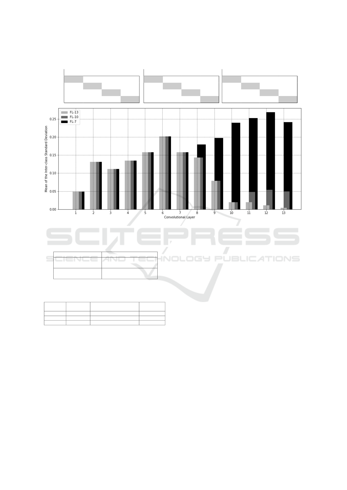
Table 6: Normalized confusion matrix FL-13, FL-10 and FL-7 experiments. The columns indicate the predict class for the

test set.

AGR FOR HRB SHR

AGR 0.3 0.26 0.26 0.19

FOR 0.01 0.99 0.00 0.00

HRB 0.26 0.21 0.23 0.30

SHR 0.20 0.29 0.23 0.28

AGR FOR HRB SHR

0.85 0.04 0.09 0.02

0.03 0.73 0.05 0.18

0.01 0.00 0.94 0.05

0.01 0.00 0.24 0.75

AGR FOR HRB SHR

0.99 0.01 0.00 0.00

0.00 0.97 0.01 0.02

0.00 0.01 0.99 0.01

0.00 0.01 0.03 0.96

Figure 4: Mean of the inter-class standard deviation (M

) in each convolutional layer for the FL-(13,10 and 7) experiments.

Table 7: Training time comparison when varying some hy-

perparameters using Intel MKL-DNN.

Hyperparameter Values

# Intra-op 20 48 19 12

# workers (k) 1 2 5 8

Simul. Batch Size (kn) 32 64 160 384

Training Time (min) 1598 903 37 69

Table 8: Comparison to baselines and deep learning models

for the test set.

Technique

Weighted

Accuracy

Technique

Weighted

Accuracy

CCV 80.6 ± 2.3% BIC 85.5 ± 1.4%

GCH 80.1 ± 2.4% Fine Tuning (original paper) 90.54 ± 1.8%

UNSER 80.3 ±0.2% Fine Tuning (FL-7) 97.1 ± 1.1%

mentation and the VGG-16 network in having ﬁxed

parameters such as pooling size and convolution ﬁl-

ter size. In this way, with the change of the other

hyperparameters, the impacts of these variations are

more effectively realized, resulting in a satisfactory

ﬁne-tuning.

5 CONCLUSIONS AND FUTURE

WORK

This paper used methods that have helped convolu-

tional networks to learn more effectively the speciﬁc

characteristics of vegetative species groups. The data

augmentation method was essential in achieving ef-

fective accuracy by balancing the data to prevent over-

ﬁtting, while transfer learning accelerated the training

process of the network, smartly, by skipping training

steps. The ﬁne-tuning approach enabled to truncate

any layers of the transfer-learning network and the

insertion of convolutional layers, to distinguish the

classes with higher accuracy. The statistical analy-

sis proposed helps to choose which layers should be

frozen avoiding unnecessary extra experimental tests

for the correct choice.

The distributed learning (training the model by di-

viding the dataset between workers) and the tuning of

the parallel operators (LSBO parameters) have shown

the possibilities to train a convolutional network in a

CPU with high training speed. It is relevant to notice

that the maximum number of workers that resulted in

good performance is limited, perhaps due to the small

dataset.

The ﬁnal result which indicates an accuracy of

about 97% is relevant for applications involving

remote sensing for the classiﬁcation of vegetation

species whose images are derived from satellites.

The classiﬁcation model implemented may not

work well if the camera is not multispectral, being an

essential equipment for the plant classiﬁcation task.

Improving Transfer Learning Performance: An Application in the Classiﬁcation of Remote Sensing Data

181

Also, for satisfactory training and inference results,

the dataset must be divided into small tiles to reduce

the number of classes present in each image.

The theoretical and experimental study of solu-

tions for implementing a classiﬁer using unbalanced

data have great importance for future work, since

most environmental monitoring applications rely on

disproportionate class data. It is intended to apply

the concepts and experiences learned in new datasets

with more classes and more data. Also, for future

work, pixel-wise semantic segmentation deep learn-

ing models (Badrinarayanan et al., 2015; Chen et al.,

2018; Ronneberger et al., 2015) may be used to clas-

sify the plants species which makes it possible to clas-

sify whole images containing multiple classes at the

same time and without being necessary to crop them

into small tiles.

ACKNOWLEDGEMENT

This work was partially funded by a Masters Scholar-

ship supported by the National Council for Scientiﬁc

and Technological Development (CNPq) at the Pon-

tiﬁcal University Catholic of Rio de Janeiro, Brazil.

REFERENCES

Aitkenhead, M., Dalgetty, I., Mullins, C., McDonald, A.

J. S., and Strachan, N. J. C. (2003). Weed and crop dis-

crimination using image analysis and artiﬁcial intelli-

gence methods. Computers and electronics in Agri-

culture, 39(3):157–171.

Badrinarayanan, V., Kendall, A., and Cipolla, R. (2015).

Segnet: A deep convolutional encoder-decoder ar-

chitecture for image segmentation. arXiv preprint

arXiv:1511.00561.

Chawla, N. V., Bowyer, K. W., Hall, L. O., and Kegelmeyer,

W. P. (2002). Smote: synthetic minority over-

sampling technique. Journal of artiﬁcial intelligence

research, 16:321–357.

Chen, L.-C., Papandreou, G., Kokkinos, I., Murphy, K., and

Yuille, A. L. (2018). Deeplab: Semantic image seg-

mentation with deep convolutional nets, atrous convo-

lution, and fully connected crfs. IEEE transactions on

pattern analysis and machine intelligence, 40(4):834–

848.

Cires¸an, D. C., Meier, U., Gambardella, L. M., and Schmid-

huber, J. (2010). Deep, big, simple neural nets for

handwritten digit recognition. Neural computation,

22(12):3207–3220.

Goyal, P., Doll

ar, P., Girshick, R., Noordhuis, P.,

Wesolowski, L., Kyrola, A., Tulloch, A., Jia, Y., and

He, K. (2018). Accurate, large minibatch sgd: training

imagenet in 1 hour. arXiv preprint arXiv:1706.02677.

Gu, J., Wang, Z., Kuen, J., Ma, L., Shahroudy, A., Shuai, B.,

Liu, T., Wang, X., Wang, G., Cai, J., et al. (2018). Re-

cent advances in convolutional neural networks. Pat-

tern Recognition, 77:354–377.

He, K. and Sun, J. (2015). Convolutional neural networks

at constrained time cost. In Proceedings of the IEEE

conference on computer vision and pattern recogni-

tion, pages 5353–5360.

He, K., Zhang, X., Ren, S., and Sun, J. (2016). Deep resid-

ual learning for image recognition. In Proceedings of

the IEEE conference on computer vision and pattern

recognition, pages 770–778.

Horler, D., DOCKRAY, M., and Barber, J. (1983). The red

edge of plant leaf reﬂectance. International Journal

of Remote Sensing, 4(2):273–288.

Jolliffe, I. (2011). Principal component analysis. In In-

ternational encyclopedia of statistical science, pages

1094–1096. Springer.

Krizhevsky, A., Sutskever, I., and Hinton, G. E. (2012). Im-

agenet classiﬁcation with deep convolutional neural

networks. In Advances in neural information process-

ing systems, pages 1097–1105.

Liu, G. and Gifford, D. (2017). Visualizing feature maps in

deep neural networks using deepresolve a genomics

case study. ICML Visualization Workshop.

Maaten, L. v. d. and Hinton, G. (2008). Visualizing data

using t-sne. Journal of machine learning research,

9(Nov):2579–2605.

Nogueira, K., Dos Santos, J. A., Fornazari, T., Silva, T. S. F.,

Morellato, L. P., and Torres, R. d. S. (2016). Towards

vegetation species discrimination by using data-driven

descriptors. In Pattern Recogniton in Remote Sens-

ing (PRRS), 2016 9th IAPR Workshop on, pages 1–6.

IEEE.

Pass, G., Zabih, R., and Miller, J. (1997). Comparing im-

ages using color coherence vectors. In Proceedings of

the fourth ACM international conference on Multime-

dia, pages 65–73. ACM.

Refaeilzadeh, P., Tang, L., and Liu, H. (2009). Cross-

validation. In Encyclopedia of database systems,

pages 532–538. Springer.

Ronneberger, O., Fischer, P., and Brox, T. (2015). U-net:

Convolutional networks for biomedical image seg-

mentation. In International Conference on Medical

image computing and computer-assisted intervention,

pages 234–241. Springer.

Russakovsky, O., Deng, J., Su, H., Krause, J., Satheesh, S.,

Ma, S., Huang, Z., Karpathy, A., Khosla, A., Bern-

stein, M., et al. (2015). Imagenet large scale visual

recognition challenge. International Journal of Com-

puter Vision, 115(3):211–252.

Simonyan, K., Vedaldi, A., and Zisserman, A. (2013).

Deep inside convolutional networks: Visualising im-

age classiﬁcation models and saliency maps. arXiv

preprint arXiv:1312.6034.

Stehling, R. O., Nascimento, M. A., and Falc

ao, A. X.

(2002). A compact and efﬁcient image retrieval ap-

proach based on border/interior pixel classiﬁcation. In

Proceedings of the eleventh international conference

ICAART 2019 - 11th International Conference on Agents and Artiﬁcial Intelligence

182

on Information and knowledge management, pages

102–109. ACM.

Swain, M. J. and Ballard, D. H. (1991). Color indexing.

International journal of computer vision, 7(1):11–32.

Szegedy, C., Liu, W., Jia, Y., Sermanet, P., Reed, S.,

Anguelov, D., Erhan, D., Vanhoucke, V., and Rabi-

novich, A. (2015). Going deeper with convolutions.

In Proceedings of the IEEE conference on computer

vision and pattern recognition, pages 1–9.

Unser, M. (1986). Sum and difference histograms for tex-

ture classiﬁcation. IEEE transactions on pattern anal-

ysis and machine intelligence, (1):118–125.

Improving Transfer Learning Performance: An Application in the Classiﬁcation of Remote Sensing Data

183