Fast and Simple Model
For Free Hanging, Pre-impregnated Carbon Fibre Material
Ole W. Nielsen, Christian Schlette and Henrik G. Petersen
The Maersk Mc-Kinney Moller Institute, University of Southern Denmark, Campusvej 55, 5230 Odense M, Denmark
Keywords:
Modeling Shapes of Deformable Objects, Robotic Layup of Fiber Plies.
Abstract:
Automated one-of-a-kind grasping and draping of pre-impregnated (prepreg) fiber plies onto complex molds
is a hitherto unsolved problem. In the project FlexDraper, we have gathered an international consortium with
industrial keyplayers for addressing this gap. Our approach is based on model- and simulation-based control
of the shaping of the plies during the draping procedure, which requires fast computable models in the draping
control loop. In this paper, we present such a fast computable mathematical model for the shape of free hanging
prepreg fiber plies with perpendicular fiber directions, where the ply is held (clamped) at a set of locations that
are not too far apart. Rather than using expensive physically based models, e.g. FEM simulations, our model is
only based on interpolations between the held locations satisfying curve length constraints in fiber directions.
The paper also contains experimental tests for the accuracy of the model.
1 INTRODUCTION
At SDU Robotics, we aim for transferring our exam-
ples from research to actual applications by building
up close cooperations with industrial partners, such
as Terma A/S, a Danish manufacturer of aerostructu-
res from carbon fiber. Despite many attempts to auto-
mate it, draping of weaved pre-impregnated (prepreg)
carbon fiber plies is a process that is - at least for low
volume production - still performed manually. Au-
tomation of these processes would lead to huge eco-
nomic benefits in many application domains, such as
aerospace, automotive and offshore energy. To make
such a system feasible, it has to be able to handle a
large variety of plies as well as parts. Theoretically,
with a proper draping tool, a trained operator will be
able to teach/program a robot to layup the plies for a
single part through experimentation. However, as we
require a large variety of parts as well as plies, and
that the quantity of each part is low, the time required
for an operator working on the robot will lead to an in-
feasible solution with respect to ROI. Hence, we need
to be able to deploy model-based automatic control of
the draping process.
In the project FlexDraper (Ellekilde et al., 2018),
we have gathered an international consortium for de-
veloping a new drape tool mounted on a conventional
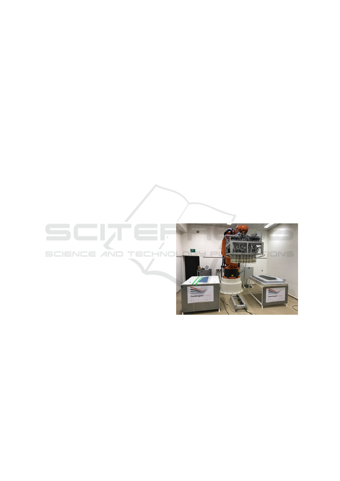
6-axis robot. The drape tool (see Figure 1) consists
of an array of suction cups where the up-down mo-
Figure 1: The FlexDraper robot.
vement of each suction cup is individually controlla-
ble. At the fixed platform, a universal joint is placed
and there is spherical joint at the cup (see Figure 2(a)).
The nearest neighbour cups are connected by rigid in-
terlinks with spherical joints at the end (see Figure
2(b)). This allow us to control the shape of fiber plies
so that we can shape them to the form of the mould.
However, one of the main issues with developing
model-based control is that the shape of the materi-
als between the suction cups needs to be accurately
estimated to enable a draping "from one side" so that
undesired air bubbles are avoided. Our approach to
model-based control is thus deploying an accurate and
Schlette C., Nielsen O. and Petersen H.
Fast and Simple Model - For Free Hanging, Pre-impregnated Carbon Fibre Material.
DOI: 10.5220/0007239700000000
In Proceedings of the 15th International Conference on Informatics in Control, Automation and Robotics (ICINCO 2018), pages 7-14
ISBN: 978-989-758-321-6
Copyright
c
 2018 by SCITEPRESS – Science and Technology Publications, Lda. All rights reserved

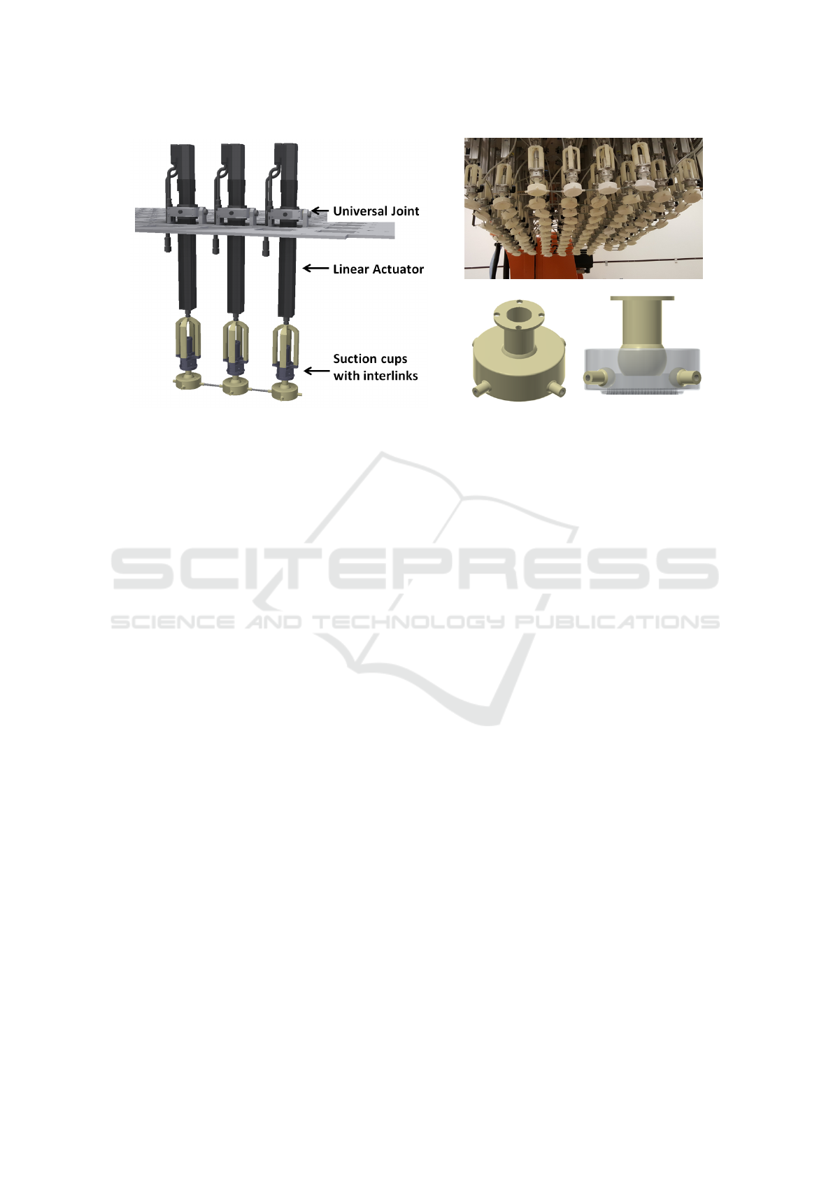
(a) Subset of tool showing the relative placement of the uni-
versal joints, actuators and suction cups.
(b) Close-up of suction cups with ball joints for
connecting with the actuator and interlink struc-
ture.
Figure 2: Actuation and suction cup design.
fast computable model for simulating the draping pro-
cess. The model must be fast computable because the
simulations are used to annotate the outcome of a stu-
died draping strategy. These annotations are used in
a simulation-based learning procedure. Hence, many
simulations must be carried out for fine-tuning the pa-
rameters of each draping process. One of the key ele-
ments is a fast computable model for predicting the
shape of the free hanging parts of the material (i.e. be-
tween the suction cups and before touching the mold).
It is the main purpose of this paper to present our solu-
tion to this and some initial experimental verifications
of its accuracy.
The paper is organized as follows: In Section 2,
we outline the properties of the FlexDraper tool for
draping and discuss the properties of the fiber ply ma-
terial and in Section 3, we discuss the organization
of the draping process. These discussions include the
desired properties of our model. Related modelling
work is discussed in Section 4 and in Section 5, we
present the model, which is the core contribution of
this paper. In Section 6, we discuss preliminary vali-
dation results and Section 7 concludes the paper.
2 THE FlexDraper TOOL AND
MATERIAL
In the FlexDraper project, a drape tool to handle the
material has been created. The tool consists of 48
suction cups arranged in a grid like structure, where
all the suction cups are connected by interlinks to
the nearest neighbours (see Figure 2(b)). The sucti-
ons cups are spaced in a loose grid roughly 11 cm
apart in both, x and y directions. This gives rise to
many small square segments or elements of free han-
ging material with sizes around 7×7cm
2
between four
suction cups and strips of free-hanging material of si-
zes around 4 × 7cm
2
between two nearest neighbor
cups (see Figure 4). It should be mentioned that alt-
hough the tool is constrained by the interlink struc-
ture, it has many passive degrees of freedom that al-
lows the suction cups to align with the mold.
The material is as mentioned a bi-directional car-
bon fiber weave, pre-impregnated with epoxy resin.
It is virtually in-extensible in the perpendicular fiber
directions but has a small slack in the weave. Further-
more, the pre-impregnation of the material means it
is ”sticky/tacky” in nature and relatively stiff with re-
spect to bending curvature and furthermore dynamic
responses (vibrations) are very small.
We therefore make the following assumptions about
the material in our model
• Since the material is relatively stiff with respect to
bending and because the distance between neig-
hbor suction cups is small, we can neglect gravity.
For the same reasons, we can assume that the ma-
terial is continuous differentiable everywhere
• Since the material is very damped, we can use an
equilibrium model
• We assume that the material is unstretchable in the
fiber directions

Figure 3: The process: Components in the FlexDraper Sy-
stem (Blue = flow of actions, green = sensor systems, red =
data and computational models).
3 THE PROCESS AND MODEL
REQUIREMENTS
The process flow is shown in Figure 3. The plies
are picked with suction cups from a flat surface. We
assume for simplicity of the model description that
the suction cup array aligns with the fibre directions.
From the tool state sensor, we have accurate predicti-
ons of the positions of all suction cups at pick up. Af-
ter pick up, the suction cups are moved to shape the
ply into what we call a preshape. With a preshaped
model, each suction cup has a position and orienta-
tion which we can again accurately predict using the
tool state sensor.
The plies are draped onto the mold by choosing
a suitable starting point (choice is depending of the
shape of the mold). Then the first suction cup with
the material attached is placed on the mold. Subse-
quently, the other suction cups are placed in a wave
like pattern running from the starting point to the
boundary. To avoid undesired air bubbles, it is very
important that also the material is attaching to the
mold sequentially from the starting point and out-
wards. To ensure this, we have at any point in time
the following available information
• The three dimensional shape of the mold surface
• The configuration of the robot
• The configuration of all the linear actuators con-
trolling the up-down movements of the suction
cups
We then have an dynamics based forward kinematics
model of the drape tool that accurately predicts the
position and orientation of all the suction cups after
the relatively small movements from the sensor mea-
sured preshape. To finalize the simulation model used
for learning, we then just need to be able to predict the
shape of the free-hanging ply material between the
suction cups. Before going into the detailed descrip-
tion of the shape predicting model, we will discuss
the learning procedure because it impacts the desired
property of the model. In the most general sense, a
draping procedure is a coordinated movement of the
robot and the linear actuators, i.e. a path in 48+6 = 54
dimensional space. To learn such a general trajectory
in 54-dimensional space is computationally infeasi-
ble. Hence, we divide the learning into a sequence
part and a trajectory part. The sequence part learning
selects the starting point and the wave pattern for pla-
cing the suction cups. The trajectory part learning de-
rives - for each step in the sequence - the trajectories
of the relevant suction cups, which are those to be pla-
ced next and their neighbours. For the sequence part,
there is in practise typically only around 5-10 relevant
options, so the main task is the derivation of the tra-
jectory part.
With the learning procedure in mind, we have the
following desired properties of the model
• It must be fast computable to allow many simula-
tions during learning
• It should be local so that a given region relevant
for a step in sequence can be simulated indepen-
dent of the rest of the ply
• The model must be accurate enough with respect
to reality to allow for simulation-based learning
4 RELATED WORK
Modelling of composite materials is a broad topic and
therefore we will only be able to give a rather sparse
overview of some of the more detailed strategies. In
the work by (Lin et al., 2012), the physical proper-
ties are modelled not only for the cloth as a whole
but also the interactions between fibers. In (Newell
and Khodabandehloo, 1995), the authors have defined
a simplified mathematical model using finite element
analysis to model deformations of plies, which is then
used to control the handling trajectories of an automa-
ted composite manufacturing facility. More recently,
(Krogh et al., 2017) used a finite element approach as
part of the Flexdraper project. The calculation time

for simulating a drape using these type of methods is
typically in the order of hours on a conventional com-
puter. Finite difference modelling is another interes-
ting approach used by (Do et al., 2006) to calculate
deformation profiles of rectangular composite plies
under the effect of multiple suction surfaces. Their
results show good correspondence between expected
results and simulations. They illustrate the impor-
tance of mesh vs accuracy vs computation time. In or-
der to reach high accuracies their computational time
was close to 30 minutes, whereas medium accura-
cies could be obtained with computational time in the
range of 10 seconds. These physics based methods
however all have a tendency of being computationally
expensive. Therefore, we look a bit broader for fast
modeling of deformable objects. Mass Spring Mo-
dels is a typical approach (see e.g.(Kot et al., 2014))
where the approach is outlined in a nice detail. The
paper (Liu et al., 2013) focuses more on the speed
of the method. More advanced versions were presen-
ted in e.g. (Zhou et al., 2008) where cloth anima-
tion using mass spring models with dynamic stiffness
is presented. The focus is on obtaining buckling and
wrinkling. Mass spring models are relatively fast dy-
namical approximations, however for the material we
are working with, the springs coefficients would be
very high. Therefore timesteps for modelling would
be very low and overall the model would hence again
become computationally expensive. There has there-
fore been a lack of computationally fast and accurate
model for prepreg fiber plies.
5 THE MODEL
In this section, we use the following notational con-
ventions: a, b, c are used for scalars, a, b, c are [3x1]
vectors in x,y,z and A, B, C are [3x3] matrices. As
mentioned, the input to our system are the positions
and orientations of all the suction cups. We just need
to derive formulas for the region around four suction
cups as illustrated in Figure 4.
The first step is to model a fiber held by two
suction cups. Using the assumption that the fiber di-
rection is aligned with the suction cup array, as well as
the information that the fiber ply was picked up from a
flat configuration, it can be reasoned that a fiber runs
from ”Point 1” to ”Point 2” in Figure 4. Similarly
the fibers run along the other solid lines in Figure 4.
To start defining the deflection model, we introduce
a function r
iξ j
(ξ), where i is the suction cup number,
ξ ∈ {s, t} is the location along the line and j indicates
which spline, with numbers 1 and 2 located as indi-
cated on the figure. The function r
iξ j
(ξ) is hence a
Figure 4: Scheme of cups on ply.
Figure 5: Model prediction for segment with 4 suction cups.
function of either s or t, and is defined in the interval
[0, L
s j
] and [0, L
t j
] for r
is j
(s) and r
it j
(t) respectively.
For a given 3D position and orientation of the four in-
volved suction cups, the vector r
iξ j
(ξ) defines the mo-
del prediction of the 3D location of the point (i, ξ, j)
on the line. It is derived in Section 5.1
Using the assumption of continuity, the region
spanned by the points 1-4 in Figure 4 can be approx-
imated by linearly interpolating between r
1s1
(s) and
r
1s2
(s). The function describing this interpolation is
called ρ
iξ
(s, t) and is a function (derived in Section
5.2) of both s and t, where i and ξ are inherited from
the r
iξ j
(ξ) function. ρ
1s
is a function in t for a given s,
defined for t ∈ [−d, d] and s ∈ [0, L
s
].
As a last step the area spanned by the points 3-
6 in Figure 4 can be approximated by performing a
polynomial fit between ρ
1s
(s, t) and ρ
3s
(s, t), as well
as performing polynomial fit between ρ
1t
(s, t) and
ρ
2t
(s, t). These functions are referred to as γ
ξ
(s, t),
where ξ is inherited from ρ
iξ
(ξ). To achieve first or-
der continuity everywhere, these two polynomial fits
are combined using a weight function, denoted w, re-
sulting in γ(s, t). The derivation of these functions
can be found in Section 5.3.

5.1 Derivation of r
Consider first as an example r
1s1
(s). Given that the
suction cups position and rotation are well known,
and that the material is continuous differentiable, the
following boundary conditions apply
r
1s1
(0) = T
1
(d, −d, 0)
0
+ (X
1
, Y
1
, Z
1
)
0
(1)
r
1s1
(L
s
) = T
2
(−d, −d, 0)
0
+ (X
2
, Y
2
, Z
2
)
0
(2)
r
0
1s1
(0) = T
1
(1, 0, 0)
0
(3)
r
0
1s1
(L
s
) = T
2
(1, 0, 0)
0
(4)
where the vector (X
i
, Y
i
, Z
i
)
0
is the center position of
suction cup i on the suction surface wrt. a global coor-
dinate frame aligned with the pick position and T
i
is
the rotation of the suction cup relative to the global
frame i.
We will have the same types of boundary condi-
tions for all the r
is j
(s) and r
it j
(t). Hence, our general
problem is to find a function r(x) satisfying
r(0) = r
0
(5)
r(L
x
) = r
L
x
(6)
r
0
(0) = r
0
0
(7)
r
0
(L
x
) = r
0
L
x
(8)
Having four boundary conditions, the simplest choice
for a continuous function will be a cubic polynomial.
r(x) = a
0
3
x
3
+ a
0
2
x
2
+ a
0
1
x + a
0
0
(9)
Assuming independence between
{
x, y, z
}
the a
0
s are
given as follows
a
0
0
= r
0
(10)
a
0
1
= r
0
0
(11)
a
0
2
=
3(r
L
x
− r
0
) − L
x
(2r
0
0
+ r
0
L
x
)
L
2
x
(12)
a
0
3
=
−2(r
L
x
− r
0
) + L
x
(r
0
0
+ r
0
L
x
)
L
3
x
(13)
The polynomial in Eq. 9 does not take care of the in-
extensibility of the fibers. To deal with that boundary
condition, another term is added to the polynomial
r
L
x
(x) = r(x) + a
0
4
dx
2
(L
x
− x)
2
(14)
The extra term a
0
4
dx
2
(L
x
− x)
2
will have no influence
on the previously derived a
0
0
to a
0
3
, as both the value
and its derivative is 0 at x = 0 and x = L
x
. It is impor-
tant to note that a
0
0
to a
0
3
are vectors in x,y,z whereas
a
0
4
is a scalar. For reasons below, we choose the term
d as
d = r(
L
x
2
) −
1
2

r(0) + r(L
x
)

(15)
To compute a
0
4
, we use that the arc length is given by
L
x
≡
Z
L
x
0
q
r
0
L
x
(x)
2
dx (16)
In order to keep these derivations at an analytical level
Eq. 16 is manipulated slightly
L
x
=
Z
L
x
0
q
1 + (r
0
L
x
(x)
2
− 1)dx (17)
under the assumption that r
0
(x)
2
is relatively close to
1, a series expansion around 1 is performed.
√
1 + x ≈ 1 +
1
2
x (18)
Resubsituting gives
L
x
≈
Z
L
x
0
(
1
2
+
1
2
r
0
L
x
(x)
2
)dx
=
L
x
2
+
1
2
Z
L
x
0



r(x) + a
0
4
dx
2
(L
x
− x)
2



2
dx (19)
This trick makes the integrand a polynomial which
can easily be solved analytically. Inserting Eq. 9 into
Eq. 19, multiplying by
2
L
x
and reordering with respect
to a
02
4
and a
0
4
results in.
0 =
"
2
105
||d||
2
L
6
x
#
a
02
4
+
"
−
2
15
(a
0
2
·d)L
4
x
−
1
5
(a
0
3
·d)L
5
x
#
a
0
4
+ ||a
0
1
||
2
+
4
3
||a
0
2
||
2
L
2
x
+ 3(a
0
2
·a
0
3
)L
3
x
+
9
5
||a
0
3
||
2
L
4
x
+ 2(a
0
1
·a
0
2
)L
x
+ 2(a
0
1
·a
0
3
)L
2
x
− 1 (20)
Eq. 20 can be redefined as
αa
02
4
+ βa
0
4
+ γ = 0 (21)
Hence the solutions are
a
0
4
=
−β ±
p
β
2
− 4αγ
2α
(22)
This will produce two solutions for a
0
4
. To choose the
correct solution, we first notice that α is positive(see
Eq.20). If γ is negative, we should extend the length.
Here we extend the length in the positive d direction.
Hence, we must choose the "+" solution. If γ is po-
sitive, we must shorten the length, and here we wish
to go in the negative d direction by choosing the least
negative of the two solutions.
This provides a full description of all the a
0
pa-
rameters in Eq.14. For simplicity in implementation
and the further derivations, Eq.14 will be redefined by
expanding the brackets and reordering with respect to
x to get a simple looking polynomial.

r
L
x
(x) = a
0
3
x
3
+ a
0
2
x
2
+ a
0
1
x + a
0
0
+ a
0
4
dx
2
(L
x
− x)
2
= (a
0
4
d)x
4
+ (a
0
3
− 2a
0
4
dL
x
)x
3
+ (a
0
2
+ a
0
4
dL
2
x
)x
2
+ a
0
1
x + a
0
0
≡ a
4
x
4
+ a
3
x
3
+ a
2
x
2
+ a
1
x + a
0
≡
4
X
k=0
a
k
x
k
(23)
Below we use the notation r
is j
(s) and a
is jk
for
r
L
x
(x) and a
k
respectively for any considered is j. Si-
milar notation is used for r
it j
(t) and a
it jk
. All these
functions and coefficients are as mentioned computed
in exactly the same way using the four end point con-
straints and the constraint on arc length.
5.2 Derivation of ρ
Similar to the previous section, the derivation will
only be detailed for ρ
1s
(s, t) as it is straightforward
to generalize to all the ρ.
Using the assumption of continuity, ρ
1s
(s, t) can
be approximated by linearly interpolating between
r
1s1
(s) and r
1s2
(s). For any given s, ρ
1s
(s, t) will have
a linear dependency in t ,that is:
ρ
1s
(s, t) = b
1s1
(s)t + b
1s0
(s) (24)
which then leads to the following conditions.
ρ
1s
(s, d) = r
1s2
(s) = b
1s1
(s)d + b
1s0
(s) (25)
ρ
1s
(s, −d) = r
1s1
(s) = −b
1s1
(s)d + b
1s0
(s) (26)
Subtracting 25 and 26 gives
b
1s1
(s) =
r
1s2
(s) − r
1s1
(s)
2d
(27)
Adding 25 and 26 gives
b
1s0
(s) =
r
1s2
(s) + r
1s1
(s)
2
(28)
Using the formulae for the r
is j
(s)’s, we get
b
1s0
(s) =
4
X
k=0
a
1s2k
− a
1s1k
2
s
k
≡
4
X
k=0
b
1s0k
s
k
(29)
and
b
1s1
(s) =
4
X
k=0
a
1s2k
− a
1s1k
2d
s
k
≡
4
X
k=0
b
1s1k
s
k
(30)
where the a
1s1k
’s were discussed in the previous
section. Complelety equivalent, we can find the
ρ
is
(s, t), b
is0
(s), b
is1
(s) for i = 3 and the ρ
it
(s, t),
b
it0
(t), b
it1
(t) for i = 1, 2.
5.3 Derivation of γ
We now consider the model of deformation in the re-
gion between the four innermost lines. We first con-
sider the curve γ
s
(s, t) interpolating between ρ
1s
(s, d)
and ρ
3s
(s, −d). The derivation of the model for γ
s
is very similar to that of r as the material is still as-
sumed first order continuous and therefore will have
both position and first derivative as boundary conditi-
ons. Similar to ρ
1s
, γ
s
is considered a function of t,
for a given s.
γ
s
(s, 0) = γ
s0
= ρ
1s
(s, d)
= b
1s1
(s)d + b
1s0
(s) (31)
γ
s
(s, L
t
) = γ
sL
t
= ρ
3s
(s, −d)
= −b
3s1
(s)d + b
3s0
(s) (32)
∂γ
s
(s, 0)
∂t
= γ
0
s0
=
∂ρ
1s
(s, d)
∂t
= b
1s1
(s) (33)
∂γ
s
(s, L
t
)
∂t
= γ
0
sL
t
=
∂ρ
3s
(s, −d)
∂t
= b
3s1
(s) (34)
the simplest choice for four boundary conditions is a
cubic polynomial in t.
γ
s
(s, t) = c
s3
(s)t
3
+ c
s2
(s)t
2
+ c
s1
(s)t + c
s0
(s) (35)
which leads to a similar solution as for r
c
s0
(s) = γ
s0
(36)
c
s1
(s) = γ
0
s0
(37)
c
s2
(s) =
3(γ
sL
t
− γ
s0
) − L
t
(2γ
0
s0
+ γ
0
sL
t
)
L
2
t
(38)
c
s3
(s) =
−2(γ
sL
t
− γ
s0
) + L
t
(γ
0
s0
+ γ
0
sL
t
)
L
3
t
(39)
Notice that as the material is not clamped at the boun-
daries, we do here not constrain the arc length to a
fixed value. Observe now that we can write
c
s j
(s) =
4
X
i=0
c
si j
s
i
(40)
where the c
si j
’s are constants. The constants can be
computed by inserting Eq. 29 and Eq. 30 and their
equivalents into the boundary conditions and subse-
quently the boundary conditions into the equations for

the c
s j
(s)’s. We get
c
si0
= db
1s1i
+ b
1s0i
(41)
c
si1
= b
1s1i
(42)
c
si2
=
3(db
3s1k
+ b
3s0k
− db
1s1k
− b
1s0k
)
L
2
t
−
2b
1s1k
+ b
3s1k
L
t
(43)
c
si3
=
2(db
3s1k
− b
3s0k
+ db
1s1k
+ b
1s0k
)
L
3
t
+
b
1s1k
+ b
3s1k
L
2
t
(44)
We then get
γ
s
(s, t) =
4
X
i=0
3
X
j=0
c
si j
s
i
t
j
(45)
Completely in an equivalent way, we derive γ
t
(s, t) as
the model of the curve between ρ
1t
(d, t) and ρ
2t
(−d, t).
Finally, to get smooth interpolations, also at the
corners, a location dependent weighted average of
γ
s
(s, t) and γ
t
(s, t) is used:
γ(s, t) =
w
t
(s, t)γ
t
(s, t) + w
s
(s, t)γ
s
(s, t)
w
s
(s, t) + w
t
(s, t)
(46)
where the weight functions are given as.
w
s
(s, t) =
ε + f (t)w(
t
L
t
) + f (s)

1 − w(
s
L
s
)

ε + f (t) + f (s)
(47)
w
t
(s, t) =
ε + f (t)

1 − w(
t
L
t
)

+ f (s)w(
s
L
s
)
ε + f (t) + f (s)
(48)
with the following sub functions
w(ξ) = 0, 5(e
−aξ
2
+ e
−a(1−ξ)
2
) (49)
f (ξ) =
ξ
L
ξ
!
k
(1 −
ξ
L
ξ
)
k
(50)
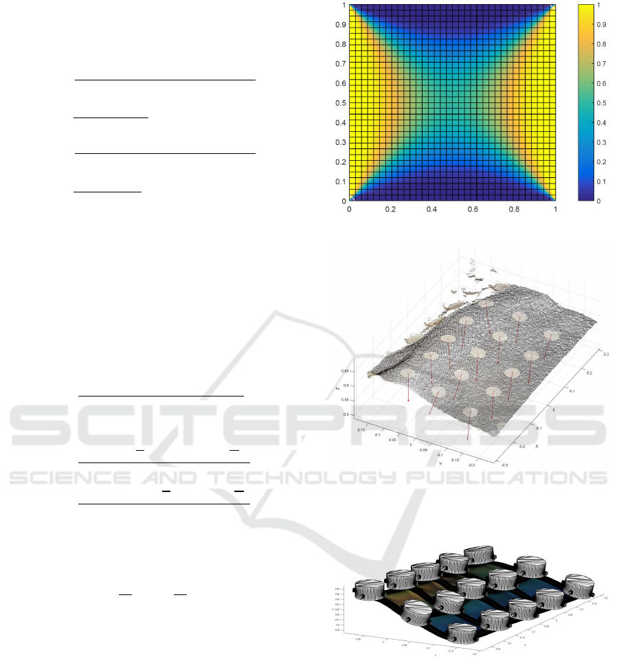
where a is a tunable parameter to adjust the
smoothness of the weighing. and ε is a small num-
ber to ensure numerical stability. A heat plot of the
weight function is shown in Figure 6.
6 VALIDATION
The test case examines the shape of a ply while being
held by an array of suction cups. We consider a sce-
nario where a full size ply was picked up from flat
surface and the suction cup configuration was resha-
ped into a typical tool-mould shape. The validation
study involves an interior region of the ply. As input
to the model, we need the L
s
and L
t
values for the
Figure 6: Overview of the 2D weight function, a = 10
4
.
Figure 7: Pointcloud captured of the material in a
held/shaped configuration. The suction cups are displayed
with white markers, the normals are shown from the suction
cup centers.
Figure 8: Model prediction of material placement when
held by suction cups as detected in Figure 7.
considered region. The current suction cups are not
optimal, so to avoid mistakes due to sliding, we esti-
mate L
s
and L
t
from the shaped configuration. To esti-
mate this arc length and filtering out noise, a NURBS
surface-fit has been performed on the point cloud seg-
ment.The suction cup positions are estimated by ma-
nually placing markers on the ply, for the vision sy-
stem to detect. These markers are also used to esti-
mate the normals of the suction cups. The vision sy-
stem is a commercially available ”Apple PrimeSense

Table 1: Summary of validation results.
RMS Error 1.6 mm
Max Error 4.6 mm
Calculation Time <1 second
Carmine 1.09”. The recorded data can be seen in
Figure.7 where as the model prediction can be seen in
Figure 8. The visualization shown in Figure 8 takes
less than one second to calculate using non optimi-
zed MATLAB code on a conventional PC. The metric
used for this evaluation only takes the offset in the ”z”
direction into account, and does not perform a one to
one mapping of points in the ply. Seen over the whole
test area (5 by 3 suction cups), the maximum devia-
tion between ply and model is 4.6 mm and the RMS
error is 1.6 mm. This is comparable to the spatial re-
solution of 1 mm for the used camera configuration.
This is already quite satisfying for the purpose of le-
arning draping strategies and with better suction cups
and camera estimates, we expect the accuracy to be
further improved.
It should however be noted that there in the test
data are some unrealistic discrepancies with respect to
suction cup positions. These test data errors give rise
to the models arc length adjustment failing on some
lines, and as a result some unexpected bulges are for-
med.
7 CONCLUSIONS AND FUTURE
WORK
In this paper, we have presented a fast computable
model for predicting the shape of prepreg fiber plies
clamped in the corners by suction cups. Our presen-
tation included a detailed derivation of the model pa-
rameters as function of the suction cup positions and
orientations. We also did some preliminary experi-
mental validations and found that the accuracy of the
model is promising. However, the quality of the expe-
rimental setting was partly insufficient and therefore
further validation in is needed.
Together with our partners, we are currently im-
proving the experimental settings by replacing the
suction cups with new versions customized for com-
posites. Furthermore, the sensor settings is being sig-
nificantly improved. Our model currently only sup-
ports completely "free hanging" regions of the ply. In
the near future, we will therefore extend the model to
include situations where part of the region between
four suction cups has made contact with the mould
and where we estimate only the shape of the remai-
ning part. This will lead to some additional issues
because we need to estimate the boundary of the free
hanging part, which will be a 3D curve and interpo-
late the shape from that boundary to the remaining 1,
2 or 3 suction cups.
ACKNOWLEDGEMENTS
This work was supported by Innovation Fund Den-
mark through the strategic platform MADE - Platform
for Future Production and the project FlexDraper.
REFERENCES
Do, D., John, S., and Herszberg, I. (2006). 3d deformation
models for the automated manufacture of composite
components. Composites Part A: Applied Science and
Manufacturing, 37(9):1377–1389.
Ellekilde, L., Wilm, J., Nielsen, O. W., Krogh, C., Glud,
J. A., Gunnarsson, G. G., Stenvang, T. S., Kristian-
sen, E., J. Jakobsen, M. K., AanÃ˛es, H., de Kruijk,
J., Sveidahl, I., Ikram, A., and Petersen, H. (2018).
An outline of the design and control of the flexdraper
robot system for automatic draping of prepreg compo-
sites fabrics. To be submitted.
Kot, M., Nagahashi, H., and Szymczak, P. (2014). Elas-
tic moduli of simple mass spring models. The Visual
Computer, pages 1–12.
Krogh, C., Glud, J. A., and Jakobsen, J. (2017). Modeling of
prepregs during automated draping sequences. In AIP
Conference Proceedings, volume 1896, pages 030–
036. AIP Publishing.
Lin, H., Ramgulam, R., Arshad, H., Clifford, M., Potluri, P.,
and Long, A. (2012). Multi-scale integrated modelling
for high performance flexible materials. Computatio-
nal Materials Science, 65:276–286.
Liu, T., Bargteil, A. W., O’Brien, J. F., and Kavan, L.
(2013). Fast simulation of mass-spring systems. ACM
Transactions on Graphics (TOG), 32(6):214.
Newell, G. and Khodabandehloo, K. (1995). Modelling
flexible sheets for automatic handling and lay-up of
composite components. Proceedings of the Institu-
tion of Mechanical Engineers, Part B: Journal of En-
gineering Manufacture, 209(6):423–432.
Zhou, C., Jin, X., Wang, C. C., and Feng, J. (2008). Plau-
sible cloth animation using dynamic bending model.
Progress in Natural Science, 18(7):879–885.