Jointly Optical Flow and Occlusion Estimation for Images with Large
Displacements
Vanel Lazcano
1
, Luis Garrido
2
and Coloma Ballester
3
1
NMFE, Universidad Mayor, Avda. Manuel Montt 318, Santiago, Chile
2
DMI, Universitat de Barcelona, Gran Via 585, Barcelona, Spain
3
DTIC, Universitat Pompeu Fabra, Roc Boronat 138, Barcelona, Spain
Keywords:
Optical Flow, Exhaustive Search, Large Displacements, Illumination Changes.
Abstract:
This paper deals with motion estimation of objects in a video sequence. This problem is known as optical
flow estimation. Traditional models to estimate it fail in presence of occlusions and non-uniform illumination.
To tackle these problems we propose a variational model to jointly estimate optical flow and occlusions.
The proposed model is able to deal with the usual drawback of variational methods in dealing with large
displacements of objects in the scene which are larger than the object itself. The addition of a term that
balances gradient and intensities increases the robustness to illumination changes of the proposed model. The
inclusion of a supplementary matching obtained by exhaustive search in specific locations helps to follow large
displacements.
1 INTRODUCTION
The apparent motion of pixels in a sequence of images
is usually called the optical flow. Optical flow compu-
tation is one of the most challenging problems in com-
puter vision, especially in real scenarios where occlu-
sions and illumination changes occur. Optical flow
has many applications, including autonomous flight
of vehicles, insertion of objects on video, video com-
pression and many others. In order to estimate this
flow field an energy model is stated, which compu-
tes the estimation error of the optical flown. Most
of the optical flow methods are grounded on the op-
tical flow constraint. This constraint is based on the
brightness constancy assumption which states that the
brightness or intensity of pixels in the image remains
constant from frame to frame along the movement of
objects. The optical flow constraint is only suitable
when the motion field is small enough or images are
very smooth.
Solving the intensity constraint is an ill-posed pro-
blem which is usually solved by adding a regularity
prior. Then the regularity prior or regularization term
added to the energy model allows defining the struc-
ture of the motion field and ensures that the optical
flow computation is well posed.
In (Horn and Schunck, 1981) was proposed to
add to the energy model a quadratic regularization
term. Actually, the work of (Horn and Schunck, 1981)
was the first one which introduced variational met-
hods to compute dense optical flow. However, the
Horn-Schunck model does not cope well with mo-
tion discontinuities, is highly sensible to noise in the
images. To tackle those drawbacks other regulariza-
tion terms have been proposed, (Nagel and Ekelman,
1986; Black and Ananda, 1996; Brox et al., 2004;
Zach et al., 2007; Werlberger et al., 2009; Sun et al.,
2010; Werlberger et al., 2010; Kr
¨
ahenb
¨
uhl and Kol-
tun., 2012; Xu et al., 2012; Chen et al., 2013; S
´
anchez
et al., 2014; Zimmer et al., 2011; Strekalovskiy et al.,
2014; Palomares et al., 2015; Ranftl et al., 2014; Sun
et al., 2014). In order to cope with large displace-
ments, optimization typically proceeds in a coarse-to-
fine manner (also called a multi-scale strategy).
Optical flow estimation using models based on
classical variational models fails if the sequence pre-
sents: i) occluded pixels, ii) displacements larger than
the size of the objects and iii) changes of illumination.
Occlusions produce lack of correspondence between
some points in the image sequence. Occluded pixels
include pixels of an image frame which are covered
by the movement of objects in the following frame.
For those occluded pixels, there is no a reliable optical
flow. In particular, the brightness constancy assump-
tion is flawed in realistic scenarios, where occlusions
occur due to the relative motion between objects in
588
Lazcano, V., Garrido, L. and Ballester, C.
Jointly Optical Flow and Occlusion Estimation for Images with Large Displacements.
DOI: 10.5220/0006716305880595
In Proceedings of the 13th International Joint Conference on Computer Vision, Imaging and Computer Graphics Theory and Applications (VISIGRAPP 2018) - Volume 5: VISAPP, pages
588-595
ISBN: 978-989-758-290-5
Copyright © 2018 by SCITEPRESS – Science and Technology Publications, Lda. All rights reserved

the scene or the camera movement, as well as illumi-
nation changes. Indeed, shadows or light reflections
that appear and move in the image sequence can also
make the brightness constancy assumption to fail.
These facts motivate us to consider an alternative
to the classical brightness constancy constraint, also
consider occlusion estimation and a new term to cope
with large displacements. In this paper we extend the
model in (Ballester et al., 2012) to a model which is
robust to illumination changes and is able to handle
large displacements.
2 RELATED WORKS
In (Zach et al., 2007) the authors present an approach
to estimate the optical flow that preserves discontinui-
ties and it is robust to noise. In order to compute the
optical flow u = (u
1
,u
2
) : Ω → R
2
between I
0
and I
1
,
the authors propose to minimize the energy
E(u) =
Z
Ω
(λ|I
0
(x) − I
1
(x + u)| + |∇u
1
| + |∇u
2
|)dx,
(1)
with a relative weight given by the parameter λ > 0.
This variational model is usually called the TV-L1 for-
mulation.
Occlusion is a challenging problem in the estima-
tion of the optical flow. Some methods implicitly deal
with occlusion by using robust norms terms in the
data term while others do an explicit occlusion hand-
ling. A first step towards taking into account occlusi-
ons was done by jointly estimating forward and bac-
kwards optical flow in (Alvarez et al., 2007). Authors
argue that at non-occluded pixels forward and bac-
kward flows are symmetric. This idea was taken by
the authors in (Ince and Konrad., 2008) and they pro-
posed to extrapolate optical flow in occluded areas.
In (Xu et al., 2012) a method to estimate occlusions
is used. They consider the fact that multiple points
mapped by the optical flow to the same point in the
following frame (collision) are likely to be occluded.
On the other hand, robustness against illumina-
tion changes would be desirable. The gradient of the
image is robust to additive illumination changes in
images (Brox et al., 2004), and therefore the gradient
constancy assumption:
∇I
0
(x) − ∇I
1
(x + u(x)) = 0,
may well be included as a new data term in a variatio-
nal energy in order to compute the optical flow u (Xu
et al., 2012).
While traditional methodology works well in ca-
ses where small structures move more or less the same
way as larger scale structures, the approach fails with
large displacement. In recent years this topic has been
tackled in interesting approaches. In (Brox et al.,
2009), a method for large displacements is proposed
that performs region-based descriptor matching. This
method estimates correctly large displacement but it
can match outliers. (Steinbruecker and Pock, 2009)
also proposes a method in order to tackle large dis-
placement. The methodology performs well in real
images with large displacements but it presents a lack
of subpixel accuracy.
To tackle large displacement (Xu et al., 2012) in-
corporates matching of SIFT features computed be-
tween images of the sequence. The fusion between
matching of SIFT features and optical flow estimation
is performed using graph cuts.
Recently new models have been proposed in order
to handle large displacements in (Weinzaepfel et al.,
2013), (Timofte and Van Gool, 2015) , (Kennedy and
Taylor, 2015), (Fortun et al., 2016) and (Palomares
et al., 2017). These models consider sparse or dense
matching using Deep matching algorithm (Weinzaep-
fel et al., 2013) or motion candidates (Fortun et al.,
2016). The principal idea is to give ”hints” to the va-
riational optical flow approach by using these sparse
matching (Weinzaepfel et al., 2013). In (Kennedy and
Taylor, 2015) and (Fortun et al., 2016) the occlusion
layer is also estimated.
3 PROPOSED MODEL
We propose a variational model for joint optical
flow and occlusion estimation, which considers color
image sequences and is able to handle illumination
changes as well as large displacements. The ingre-
dients are detailed in the following sections.
3.1 Occlusion Estimation
Inspired by (1) and (Ballester et al., 2012) we present
a joint optical flow and occlusions estimation model.
The divergence of the motion field can be used to
distinguish between different types of motion areas:
the divergence of a flow field is negative for occluded
areas, positive for dis-occluded, and near zero for the
matched areas.
Our model considers three consecutive color frames
I
−1
,I
0
,I
1
: Ω → R
3
as (Ballester et al., 2012), which
we assume to have values in the RBG color space,
hence each frame I
i
has three color components I
1
i
,
I
2
i
, I
3
i
, associated to the red, green and blue channels,
respectively. In order to compute the optical flow bet-
ween I
0
,I
1
let χ : Ω → [0, 1] be the function modeling
Jointly Optical Flow and Occlusion Estimation for Images with Large Displacements
589

the occlusion mask, so that χ = 1 identifies the occlu-
ded pixels, i.e. pixels that are visible in I
0
but not in I
1
.
Our model is based on the assumptions: (i) pixels that
are not visible in frame I
1
are visible in the previous
frame of I
0
(let I
−1
be that frame), (ii) the occluded
region given by χ = 1 should be correlated with the
region where div(u) is negative, and (iii) motion of
the occluded background area is not fast as the one
of the occluding foreground (Ballester et al., 2012).
Thus, we propose to compute the optical flow and the
occlusion mask by minimizing the energy:
E
c
(u,χ) = E
c
d
(u,χ)+E
r
(u,χ)+
η
2
Z
Ω
χ|u|
2
dx
+ β
Z
Ω
χdiv(u)dx,
where E
c
d
(u.χ) and E
r
(u,χ) are given by
E
c
d
(u,χ) =λ
3
∑
k=1
Z
Ω
((1 − χ)|I
k
0
(x) − I
k
1
(x + u(x))|
+ λ
3
∑
k=1
Z
Ω
χ|I
k
0
(x) − I
k
−1
(x − u(x))|)dx.
E
r
(u,χ) =
Z
Ω
g(x)(
|
∇u
1
|
+
|
∇u
2
|
+
|
∇χ
|
)dx, (2)
with η ≥ 0, β > 0 and g(x) =
1
1+γ
|
∇I
0
(x)
|
, x ∈ Ω, γ >
0. Notice that, if χ(x) = 0, then we compare I
k
0
(x)
and I
k
1
(x + u(x)). If χ(x) = 1, we compare I
k
0
(x) and
I
k
−1
(x − u(x)).
3.2 Robustness to Color Changes
The color constancy assumption is frequently viola-
ted due to illumination changes, shadows or reflecti-
ons. A combination of the color constancy assump-
tion and the gradient constancy assumption in the data
term seems to be a valuable approach to alleviate this
problem (Xu et al., 2012). We extend our color model
to consider a combination of intensities and gradients
by introducing an adaptive weight map α : Ω → [0,1]
that allows to balance in an adaptive way the contri-
bution of color and gradient constraints at each point
in the image domain (Xu et al., 2012). We propose
the following model:
E
c
α
(u,χ) = E
c
d,α
(u,χ)+ E
r
(u,χ)+
η
2
Z
Ω
χ|u|
2
dx + β
Z
Ω
χdiv(u)dx,
where E
c
d,α
(u,χ) can be written as:
E
c
d,α
(u,χ) =
Z
Ω
α(x)D
I,χ
(u,χ,x)
+
Z
Ω
(1 − α(x))D
∇I,χ
(u,χ,x)dx,
(3)
and D
I,χ
(u,χ,x) and D
∇I,χ
(u,χ,x) are point-wise data
costs based on the comparison of color and gradient
of the image, respectively. Roughly speaking, D
I,χ
contains the comparison kI
k
0
(x)−I
k
1
(x+u)k and D
∇I,χ
the comparison τk∇I
0
(x) − ∇I
1
(x + u)k, with τ > 0.
Then, the weight map α(x) is defined in (Xu et al.,
2012) as
α(x) =
1
1 + e
˜
β(D
I,χ
(u,x)−D
∇I,χ
(u,x))
, (4)
where
˜
β is a positive constant. Let us com-
ment about the behavior of (4). If the term
D
I,χ
(u,x)  D
∇I,χ
(u,x), the difference D
I,χ
(u,x) −
D
∇I,χ
(u,x) will be positive and the exponential value
e
˜
β(D
I,χ
(u,x)−D
∇I,χ
(u,x))
will be large. Then, α(x) will be
a small value, say near 0, and the data term will have
more confidence on the gradient constancy assump-
tion. On the other hand, if D
∇I,χ
(u,x)  D
I,χ
(u,x),
the difference D
I,χ
(u,x) − D
∇I,χ
(u,x) will be negative
and the exponential value e
˜
β(D
I,χ
(u,x)−D
∇I,χ
(u,x))
will be
very small. In other words, the data term will be more
confident on the color constancy assumption.
3.3 Large Displacements
To handle large displacements we add to our model a
term µ
R
Ω
χ
p
c(x)
|
u − u
e
|
, where u
e
is an optical flow
obtained by exhaustive search, χ
p
is a characteris-
tic function indicating location where supplementary
matching could improve the motion estimation, c(x)
is a confidence on the exhaustive matching at x and
µ > 0.
Summarising, the proposed model to handle large
displacement is:
E
c
αl
(u,χ) = E
c
d,α
(u,χ) + E
r
(u,χ)+
η
2
Z
Ω
χ|u|
2
dx + β
Z
Ω
χdiv(u)dx+
µ
Z
Ω
χ
p
c(x)
|
u − u
e
|
dx, (5)
In our implementation and for efficiency reasons, we
consider an upper bound for the expected maximum
displacement v
max
.
3.3.1 Confidence Function c(x)
We directly integrate exhaustive point corresponden-
ces into the variational model and the proposed confi-
dence measure, used to determine the weight given to
matching computed by exhaustive search, is
c(x) =

d
2
− d
1
d
1

2

E
c
dα
(u,x)
E
exha
(u
e
,x)

2
VISAPP 2018 - International Conference on Computer Vision Theory and Applications
590

where d
1
, d
2
are the distances to the first and second
best candidate respectively of the exhaustive search,
E
c
dα
(u,x) is the error defined in (3) and E
exha
(u
e
,x) is
the error of the exhaustive search. This measure was
used in (Stoll et al., 2012) to validate the correctness
of a given optical flow field at each point.
3.3.2 Construction of χ
p
In order to determine specific locations where supple-
mentary matching could improve the motion estima-
tion, we evaluate the data term, at each x ∈ Ω with
the computed flow u and the occlusion map χ. The
idea is that if the value E
c
d,α
(u,χ) is large, then the
estimation might be improved. Additionally, we con-
sider the smaller eigenvalue λ(x) of the structure ten-
sor associated to the image I
0
. With these ingredients,
the set Ω
χ
p
where supplementary matching could im-
prove motion estimation is defined as:
Ω
χ
p
=
{
x ∈ Ω
|
E
c
dα
(u,χ)(x) > θ
E
∧ λ(x) > θ
λ
}
where θ
E
and θ
λ
are given constants which we will
determine empirically and fix for the experiments we
performed. That is, if E
c
d,α
> θ
E
, then we assume
that the error is large enough to be improved using
a supplementary match. The set of points that be-
long to Ω
χ
p
define a binary mask, which we denote
by χ
p
: Ω → [0, 1].
3.4 Solving the Model
In order to minimize (5), we relax it and introduce
five auxiliary variables v
1
,v
2
,v
3
,v
4
,v
5
representing
the flow and used to decouple the nonlinear terms,
where v
1
, v
2
, v
3
correspond to the red, green and blue
channels, respectively and v
4
, v
5
correspond to ∂
x
and
∂
y
respectively. We penalize the difference between
the optical flow u and each of the auxiliary variables
v
1
, v
2
, v
3
, v
4
, v
5
. Thus, to compute the occlusions and
the optical flow between I
0
,I
1
, we propose to mini-
mize the following energy:
e
E
c
α,l
(u,χ, ˜v) = E
c
d
( ˜v,χ) + E
r
(u,χ)+
η
2
Z
Ω
χ
|
˜v
|
2
dx +β
Z
Ω
χdiv(u)dx+
1
2θ
Z
Ω
|
˜u − ˜v
|
2
dx,
(6)
where
|
˜v
|
2
stands for
5
∑
k=1
|
v
k
|
2
and
E
c
d
( ˜v,χ) =
λ
Z
Ω
(1−χ)
3
∑
k=1



ρ
k
1
(v
k
)



dx+λ
Z
Ω
χ
3
∑
k=1



ρ
k
−1
(v
k
)



dx,
and ρ
k
i
is the linearized version of I
k
0
(x) − I
k
i
(x + ε
i
v
k
)
around an approximation u
0
of u, with i = −1,1 and
ε
−1
= −1 and ε
1
= 1, and k = 1,2, 3 (corresponding
to each color channel). The linearization procedure is
applied to each ρ
k
i
(x).
We minimize
e
E
c
αl
in (6) by alternating among
the minimization with respect to each variable while
keeping the remaining fixed as (Ballester et al.,
2012),(Zach et al., 2007). In particular, the minimi-
zation of
e
E
c
αl
with respect to u, v
k
and χ is described
in the following propositions.
Proposition 1. The minimum of
e
E
c
αl
with respect to
u = (u
1
,u
2
) is given by
u
i
=
1
5
∑
5
k=1
v
i
k
+ θdiv(gξ
i
) + θβ
∂χ
∂x
i
+ µθu
i
e
χ
p
c
1 + µθχ
p
c
, (7)
with i=1,2 and u
e
= (u
1
e
,u
2
e
). ξ
1
and ξ
2
are computed
using the following iterative scheme
ξ
t+1
i
=
ξ
t
i
+
τ
u
θ
g∇(
1
5
∑
5
k=1
v
i
k
+ θdiv(gξ
t
i
) + θβ
∂χ
∂x
i
)
1 +
τ
u
θ
|g∇(
1
5
∑
5
k=1
v
i
k
+ θdiv(gξ
t
i
) + θβ
∂χ
∂x
i
)|
,
(8)
where ξ
0
i
= 0 and τ
u
≤ 1/8.
Proposition 2. Assume that χ : Ω → {0,1}. The mi-
nimum of
˜
E
c
α,l
with respect to v
k
= (v
1
k
,v
2
k
) is
v
k
=





η
i
u−µ
i
ε
i
α(x)∇I
k
i
(x
∗
) if Λ
k
i
(u)>µ
i
α(x)m
k
i
η
i
u+µ
i
ε
i
α(x)∇I
k
i
(x
∗
) if Λ
k
i
(u)<−µ
i
α(x)m
k
i
u−ε
i
ρ
k
i
(u)
∇I
k
i
(x
∗
)
|∇I
k
i
(x
∗
)|
2
if |Λ
k
i
(u)| ≤ µ
i
α(x)m
k
i
,
when i = 1 and ε
1
= 1, η
1
= 1, µ
1
= λθ, Λ
k
1
(u) =
ρ
k
1
(u) when χ = 0, and i = −1, ε
−1
= −1, η
−1
=
1
1+ηθ
, µ
−1
=
λθ
1+ηθ
, Λ
−1
(u) = ρ
k
−1
(u) +
ηθ
1+ηθ
u ·
∇I
k
−1
(x + ε
i
u
0
) when χ = 1. Additionally we create
x
∗
= x + ε
i
u
0
. The term m
k
i
was defined as m
k
i
:=
|∇I
k
i
(x
∗
)|
2
. Arguments x in u,u
0
are omitted.
Once all v
k
are computed, we define F = λA+
1
5
B,
where
A = −α(x)
3
∑
k=1



ρ
k
1



− (1 − α(x))
5
∑
k=4
|
ρ
1
(v
k
)
|
!
,
B =
5
∑
k=1
(v
k
− u)
2
!
,
and G = λC +
η
5
D, where,
C = −α(x)
3
∑
k=1



ρ
k
−1



− (1 − α(x))
5
∑
k=4
|
ρ
−1
(v
k
)
|
!
,
D =
5
∑
k=1
(v
k
)
2
!
.
Jointly Optical Flow and Occlusion Estimation for Images with Large Displacements
591

Proposition 3. Let 0 < τ
ψ
τ
χ
< 1/8. Given u,v, the
minimum
¯
χ of
˜
E
c
α
with respect to χ can be obtained by
the following primal-dual algorithm
ψ
n+1
= P
B
(ψ
n
+ τ
ψ
g ∇χ
n
)
χ
n+1
= P
[0,1]

χ
n
+ τ
χ

div(gψ
n+1
) − β divu − F − G

,
where P
B
(ψ) denotes the projection of ψ on the unit
ball of R
2
and P
[0,1]
(r) = max(min(r,1),0), r ∈ R.
3.5 Algorithm
This section is devoted to present the numerical algo-
rithm for the minimization of (6), including pseudo-
codes describing its main steps. In particular, Al-
gorithm 1 summarizes our illumination changes and
large displacement robust optical flow model presen-
ted in section 3.4. The value of α(x), for all x ∈ Ω
are updated after each propagation of the optical flow
to the finer scale, before starting the estimation of the
flow field at that scale.
The data attachment
R
c(x)χ
p
(u−u
e
)
2
depends on
the confidence value c(x), the mask χ
p
and exhaustive
matchings u
e
. The confidence value is an estimation
of the reliability of the exhaustive matchings.
4 DATABASE AND
EXPERIMENTS
We evaluate our model in two publicly databases:
Middlebury (Scharstein and Szeliski, 2002) and MPI
Sintel (Butler et al., 2012). In Figure 1, we show ima-
ges of the Middlebury dataset. These sequences con-
tain displacements larger than the size of the object
and also contain shadows and reflections. Figure 1
shows three consecutive frames of the sequence Be-
anbags(BB) and DogDance(DD). BB sequence pre-
sents balls that move while producing shadows on the
T-shirt. In DD sequence the girl moves to the right
and the dog moves to the left.
MPI database (Butler et al., 2012) presents long
synthetic sequences containing large displacements,
blur or reflections, fog and shadows. Moreover, there
are two versions of the MPI database: clean and final.
The final version is claimed to be more challenging
and we take it for our evaluation. Figure 2 displays
some examples of the MPI database. There are ima-
ges with large displacements. In the cave 4 sequence
a girl fight with a dragon moving her lance inside a
cave in (a), (b), (c). In (d), (e) and (f) the girl moves
downward a fruit on her hand.
Input : Three consecutive color frames
I
−1
,I
0
,I
1
and u
e
Output: Flow field u and occlusion layer χ
for I
0
, and α(x)
Compute down-scaled images I
s
−1
,I
s
0
,I
s
1
for
s = 1,. .., N
scales
;
Initialize u
N
scales
= v
N
scales
k
= 0, and
χ
N
scales
= 0, α
N
scales
(x) = 1.0, γ = 0;
for s ← N
scales
to 1 do
Compute α
s
(x) using (4);
for w ← 1 to N
warps
do
Compute I
s
i
(x + ε
i
u
0
(x)),
∇I
s
i
(x + ε
i
u
0
(x)), and ρ
i
, i = −1,1;
n ← 0;
while n < outer
iterations do
Compute v
k
s
using Proposition 2;
for l ← 1 to inner iterations u do
Solve for ξ
l+1,s
i
, i ∈ {1, 2},
using the fixed point
iteration (Proposition 1);
end
Compute u
s
using Proposition 1
considering data attachment
µ
R
c(x)χ
p
(u − u
e
);
for m ← 1 to inner iterations χ
do
Solve for χ
m+1
using the
primal-dual algorithm
(Proposition 3);
end
end
end
Compute E
c
dα
(x), λ(x);
Compute χ
p
(E
c
dα
(x),λ(x),θ
λ
,θ
E
) implies
Ω
χ
p
;
If s > 1 then scale-up u
s
,v
s
,χ
s
to
u
s−1
,v
s−1
,χ
s−1
;
end
u = u
1
and χ = T
µ
(χ
1
)
Algorithm 1: Algorithm for illumination changes and
large displacement robust optical flow.
5 RESULTS
For all experiments parameters are fixed to: θ = 0.40,
λ = 0.60, α = 0.0, β = 1.0, θ
λ1
= 0.98 and θ
E
= 0.98.
The µ decreased its value in each iteration with initial
value µ
o
= 300 and µ
n
= (0.6)
n
µ
0
in the following
iterations. For real images we use blocks of 7 × 7
pixels and for synthetic images we use blocks of 31 ×
31 pixels.
VISAPP 2018 - International Conference on Computer Vision Theory and Applications
592

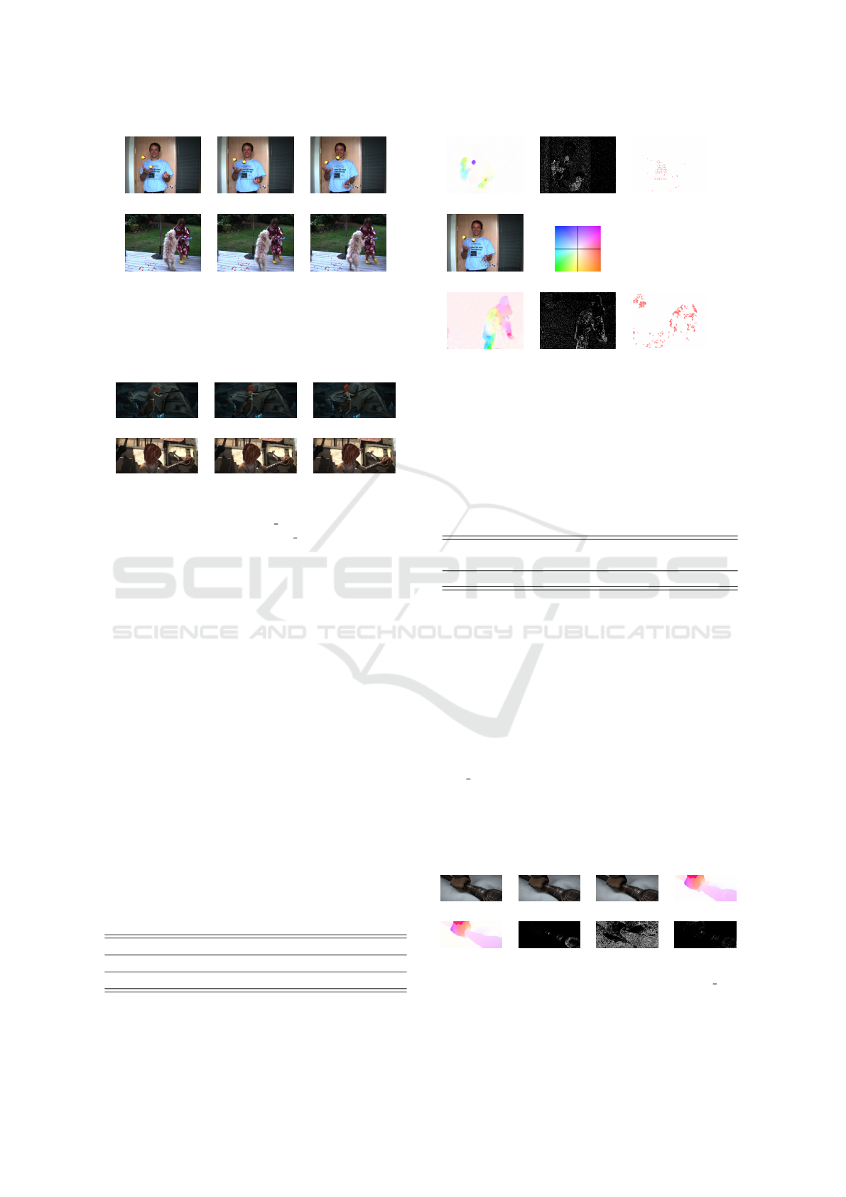
(a) (b) (c)
(d) (e) (f)
Figure 1: Middlebury BB video containing large displace-
ments, illumination changes, shadows that moves in scene.
(a) frame9, (b) frame10, (c) frame11 of the BB sequence.
(d) frame09, (e) frame10 and (f) frame11 of the DD se-
quence.
(a) (b) (c)
(d) (e) (f)
Figure 2: Images of the MPI database. (a) frame13, (b)
frame14 and (c) frame15 of cave 4 sequence. (d) frame19,
(e) frame20 and (f) frame21 of Alley 4 sequence.
Figure 3 presents the obtained results: (a) color
coded estimated optical flow for BB, (b) occluded re-
gions (let us observe how they are correctly estimated,
in particular on the face of the man), (c) χ
p
for BB (d)
the compensated image. (e) color coding scheme. (f)
encoded optical flow for DD, (g) the estimated occlu-
sion (notice that the occlusion appears in the right side
of the girl and in the left side of the dog), (h) χ
p
for
DD.
We have divided MPI database in three subsets:
large, medium and small displacements. The quanti-
tative obtained results are shown in Table 1. For large
displacements we set the parameter v
max
= 150, for
medium displacements we set v
max
= 40 and for small
displacement we set v
max
= 1. For large displacement
we set θ
λ
= 0.50 and θ
e
= 0.50, for medium and small
displacement we set θ
λ
= 0.98 and θ
e
= 0.98. The
Average End Point Error for the whole database is
presented in Table 1.
Table 1: End Point Error obtained by our model in subset:
large displacement, medium displacement and small displa-
cement of MPI.
Large Medium Small
EPE 18.82 EPE 1.41 EPE 0.80
Total Average EPE 7.17
Let us observe from Table 1 that although the
obtained average is EPE = 18.82 in Large Displace-
(a) (b) (c)
(d) (e)
(f) (g) (h)
Figure 3: Results obtained in BB and DD sequence. (a)
color coded flow field obtained by our model. (b) estima-
ted occlusion mask. (c) χ
p
. (d) Compensated image using
the occlusion mask, Compensated = (1 − χ)I
1
(x + u(x)) +
χI
1
(x − u(x)) . (e) color code for flow field. (f) color code
for DogDance sequence. (g) estimated occlusion mask. (h)
χ
p
Table 2: End Point Error obtained by our model in subset of
MPI considering displacement < 150 pixels.
Large Our
Displacement model DeepFlow MDP-Flow2
Average EPE 8.82 10.61 9.12
ment videos, the average EPE in all sequence drops to
7.17. If we only consider frames that contains displa-
cements less than 150 pixels the error drops to 8.82 in
Table 2. We also show in Table 2 results obtained by
DeepFlow in these subsets (Weinzaepfel et al., 2013)
and MDPOF (Xu et al., 2012).
In Figure 5 and Figure 4 we show qualitative re-
sults obtained for MPI data base.
In Figure 4 we have computed the optical flow be-
tween frame 27 and frame 28 of the sequence am-
bush 7, by considering three frames: frame 26 which
is considered to be I
−1
in our energy model, frame 27
which is I
0
and frame 27 is I
1
. Results are shown
in Figure 4. Original frames 26, 27 and 28 corre-
spond to subfigures (a), (c) and (e), respectively. This
sequence presents small displacement but there is a
(a) (b) (c) (d)
(e) (f) (g) (h)
Figure 4: Results obtained by our method in ambush 7 vi-
deo sequence. (a), (b) and (c): frame 26, 27 and 28, re-
spectively. (b) Optical flow ground truth. (f) Estimated op-
tical flow. (f) λ(x). (g) α(x). (h) χ(x).
Jointly Optical Flow and Occlusion Estimation for Images with Large Displacements
593

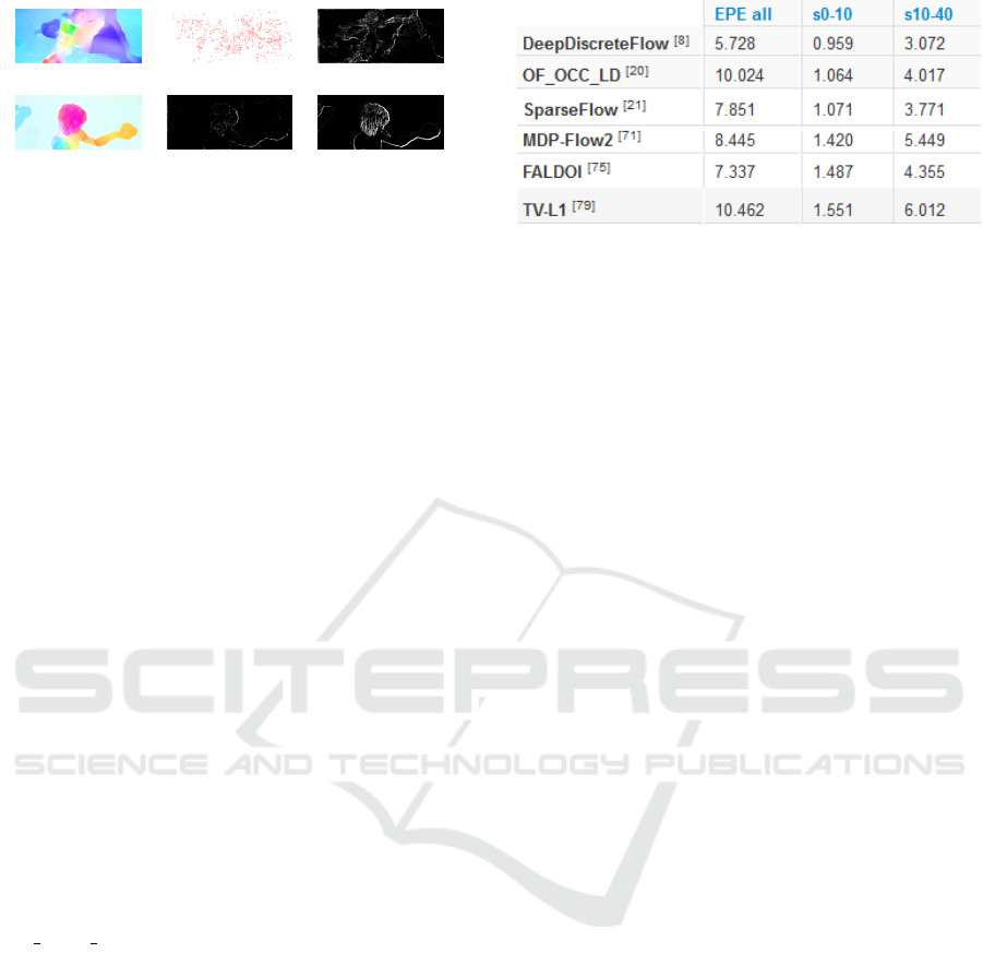
(a) (b) (c)
(d) (e) (f)
Figure 5: Images of the MPI video database. (a) color co-
ded optical flow , (b) χ
p
and (c) estimated occlusions cave4
sequence. (d) color coded optical flow, (e) estimated occlu-
sion and (f) ground truth occlusion.
shadow that moves. The lance in the image presents
small texture. This texture in the sequence presents
small variations (like noise) frame to frame. In (d)
we show the estimated optical flow. We observe that
the optical flow was robustly estimated on the snow
(where the shadow moves). In (f) we show the mini-
mum eigenvalue of the structure tensor of the frame
27. We observe that the structure lay on the small de-
tails of the lance. In (g) we show the adaptive balance
term α(x). This show that on the snow region the co-
lor constancy constrains does not holds and gradients
should be used (α(x) = 0). On the other hand where
α(x) = 1.0 intensity should be used. In (h) we have
estimated occlusions on the texture of the lace due to
this small variation frame to frame.
In Figure 5 our estimated optical flow is displayed
in (a). In (b) we show χ
p
indicating the positions
where the exhaustive search is incorporated. (c) pre-
sents the estimated occlusion layer. (d) color coded
optical flow for Alley1 sequence. (e) Estimated occlu-
sion layer. (f) ground truth occlusion layer. Compa-
ring (e) and (f) we see that they are very similar.
Figure 6 shows a comparison on MPI Sintel da-
tabase. These results are available in the Sintel web-
site (Butler et al., 2012). Our proposal is denoted as
OF OCC LD. Notice that for s0-10 our model is ran-
ked 20 (in brakets) of 110 reported method in the MPI
site. For s10-40 our method is ranked 41. Finally for
EPEall our method is ranked 97 outperforming TV-L1
which is ranked 102.
5.1 Critical Discussion
MPI test set includes small, medium and large dis-
placements (approx. 400 pixels). For small and me-
dium displacements, our method is ranked 20 and 41,
respectively. For large displacements, the position
drops to 97 which may well be due to the fact that,
for efficiency reasons, in our experiments the large
displacement threshold v
max
(which should be at least
400) was set to 150.
Figure 6: Comparative results obtained by our method in
MPI test set. EPEall is Endpoint error over the complete
frames, s0-10 error over regions with displacements lower
than 10 pixels, s0-40 error over regions with displacements
between 10 and 40 pixels.
6 CONCLUSIONS
We proposed a variational model to jointly estimate
the optical flow and the occlusion layer incorporating
the occlusion information in its energy based on the
divergence of the flow. The optical flow on visible
pixels is forward estimated and while it is backwards
estimated on occlude pixels, from three consecutive
frames. The proposed robust model handles illumi-
nations changes using a balance term between gra-
dients and intensities improving the performance of
the optical flow estimation in scenarios with illumi-
nation changes. Thanks to the use of supplementary
matches the model is able to capture large displace-
ments, even of small objects. As future work we plan
to accelerate the exhaustive matching computation in
order to avoid the v
max
restriction and handle arbitrary
largest displacements. It also includes a parallel com-
putation and GPU implementation.
REFERENCES
Alvarez, L., Deriche, R., Papadopoulo, T., and Sanchez, J.
(2007). Symmetrical dense optical flow estimation
with occlusions detection. International Journal of
Computer Vision, 75(3 ):371–385.
Ballester, C., Garrido, L., Lazcano, V., and Caselles, V.
(2012). A tv-l1 optical flow method with occlusion
detection. In DAGM/OAGM, LNCS 7476. Springer
Verlag.
Black, M. J. and Ananda, P. (1996). The robust estima-
tion of multiple motions: Parametric and piecewise-
smooth flow fields. Computer vision and image un-
derstanding, 63(1):75–104.
Brox, T., Bregler, C., and Malik, J. (2009). Large displace-
ment optical flow. In Proceedings of the IEEE Com-
puter Vision and Pattern Recognition, pages 500–513.
Brox, T., Bruhn, A., Papenberg, N., and Weickert, J. (2004).
High accuracy optical flow estimation based on a the-
VISAPP 2018 - International Conference on Computer Vision Theory and Applications
594

ory for warping. In European Conference on Compu-
ter Vision (ECCV), volume 3024, pages 25–36. Lec-
ture Notes in Computer Science.
Butler, D. J., Wulff, J., Stanley, G. B., and Black, M. J.
(2012). A naturalistic open source movie for optical
flow evaluation. In A. Fitzgibbon et al. (Eds.), editor,
European Conf. on Computer Vision (ECCV), Part IV,
LNCS 7577, pages 611–625. Springer-Verlag.
Chen, Z., Jin, H., Lin, Z., Cohen, S., and Wu, Y. (2013).
Large displacement optical flow from nearest neig-
hbor fields. In IEEE Conference on Computer Vision
and Pattern Recognition (CVPR), pages 2443–2450.
Fortun, D., Bouthemy, P., and Kervrann, C. (2016). Aggre-
gation of local parametric candidates with exemplar-
based occlusion hangling for optical flow. Computer
Vision and Image Undestanding, pages 81–94.
Horn, B. K. and Schunck, B. H. (1981). Determining optical
flow. Artificial Intelligence, 17:185–203.
Ince, S. and Konrad., J. (2008). Occlusion-aware optical
flow estimation. IEEE Transactions on Image Proces-
sing, 17(8):1443–1451.
Kennedy, R. and Taylor, C. J. (2015). Optical flow with geo-
metric occlusion estimation and fusion of multiple fra-
mes. In EMMCVPR 2015, Hong Kong, China, Janu-
ary 13-16, 2015. Proceedings, pages 364–377. Sprin-
ger International Publishing.
Kr
¨
ahenb
¨
uhl, P. and Koltun., V. (2012). Efficient nonlocal
regularization for optical flow. In European Confe-
rence on Computer Vision (ECCV), pages 356–369.
Springer.
Nagel, H.-H. and Ekelman, W. (1986). An investigation
of smoothness constraints for the estimation of displa-
cement vector fields from image sequences. Pattern
Analysis and Machine Intelligence, 6(5):565–593.
Palomares, R. P., Haro, G., and Ballester, C. (2015).
A rotation-invariant regularization term for optical
flow related problems. Lectures Notes in Computer
Science, 9007:304–319.
Palomares, R. P., Meinhardt-Llopis, E., Ballester, C., and
Haro, G. (2017). Faldoi: A new minimization strategy
for large displacement variational optical flow. Jour-
nal of Mathematical Imaging and Vision, 58(1):27–
46.
Ranftl, R., Bredies, K., and Pock, T. (2014). Non-local total
generalized variation for optical flow estimation. In
Computer Vision–ECCV, pages 439–454. Springer.
S
´
anchez, J., Salgado, A., and Monz
´
on, N. (2014). Preser-
ving accurate motion contours with reliable parameter
selection. In IEEE International Conference on Image
Processing (ICIP), pages 209–213.
Scharstein, S. and Szeliski, R. (2002). A taxonomy and
evaluation of dense two-frame stereo correspondence
algorithms. International journal of computer vision,
47 :7–42.
Steinbruecker, F. and Pock, T. (2009). Large displacement
optical flow computation without warping. In Interna-
tional Conference on Computer Vision, pages 1609–
1614.
Stoll, M., Volz, S., and Bruhn., A. (2012). Adaptive in-
tegration of features matches into variational optical
flow methods. In Proc. of the Asian Conference in
Computer Vision (ACCV), pages 1–14.
Strekalovskiy, E., Chambolle, A., and Cremers, D. (2014).
Convex relaxation of vectorial problems with coupled
regularization. SIAM J. Imaging Sciences, 7(1 ):294–
336.
Sun, D., Roth, S., and Black, M. J. (2010). Secrets of opti-
cal flow estimation and their principles. In IEEE Con-
ference on Computer Vision and Pattern Recognition,
pages 2432–2439.
Sun, D., Roth, S., and Black, M. J. (2014). A quantitative
analysis of current practices in optical flow estimation
and the principles behind them. International Journal
of Computer Vision, 2 (106):115–137.
Timofte, R. and Van Gool, L. (2015). Sparse flow: Sparse
matching for small to large displacement optical flow.
IEEE WACV, 00:1100–1106.
Weinzaepfel, P., Revaud, J., Harchaoui, Z., and Schmid, C.
(2013). Deepflow: Large displacement optical flow
with deep matching. In IEEE International Confe-
rence on Computer Vision, Sydney, Australia, pages
1385–1392.
Werlberger, M., Pock, T., and Bischof, H. (2010). Mo-
tion estimation with non-local total variation regula-
rization. In IEEE Conference on Computer Vision and
Pattern Recognition(CVPR), pages 2464–2471.
Werlberger, M., Trobin, W., Pock, T., Wedel, A., Cremers,
D., and Bischof, H. (2009). Anisotropic huber-l1 op-
tical flow. In Proceedings of the BMVC.
Xu, L., Jia, J., and Matsushita, Y. (2012). Motion detail
preserving optical flow estimation. In Pattern Analy-
sis and Machine Intelligence, IEEE Transactions on,
volume 34, pages 1744–1757.
Zach, C., Pock, T., and Bischof, H. (2007). A duality
based approach for realtime tv-l1 optical flow. In
Proceedings of the 29th DAGM Conference on Pat-
tern Recognition, pages 214–223. Berlin, Heidelberg,
Springer-Verlag.
Zimmer, H., Bruhn, A., and J., W. (2011). Optic flow in
harmony. International Journal of Computer Vision,
93(3):368–388.
Jointly Optical Flow and Occlusion Estimation for Images with Large Displacements
595