
Deriving Realistic Mathematical Models from Support Vector
Machines for Scientific Applications
Andrea Murari
1
, Emmanuele Peluso
2
, Saeed Talebzadeh
2
, Pasqualino Gaudio
2
, Michele Lungaroni
2
,
Ondrej Mikulin
3
, Jesus Vega
4
and Michela Gelfusa
2
1
Consorzio RFX (CNR, ENEA, INFN, Università di Padova, Acciaierie Venete SpA),
Corso Stati Uniti 4, 35127 Padova, Italy
2
Associazione EURATOM-ENEA, University of Rome “Tor Vergata”, Roma, Italy
3
Institute of Plasma Physics AS CR, ZaSlovankou 3, Prague, Czech Republic
4
Asociación EURATOM/CIEMAT para Fusión, Avda. Complutense, 22. 28040, Madrid, Spain
Keywords: Machine Learning Tools, Support Vector Machines, Symbolic Regression, Genetic Programming.
Abstract: In many scientific applications, it is necessary to perform classification, which means discrimination
between examples belonging to different classes. Machine Learning Tools have proved to be very
performing in this task and can achieve very high success rates. On the other hand, the “realism” and
interpretability of their results are very low, limiting their applicability. In this paper, a method to derive
manageable equations for the hypersurface between classes is presented. The main objective consists of
formulating the results of machine learning tools in a way representing the actual “physics” behind the
phenomena under investigation. The proposed approach is based on a suitable combination of Support
vector Machines and Symbolic Regression via Genetic Programming; it has been investigated with a series
of systematic numerical tests, for different types of equations and classification problems, and tested with
various experimental databases. The obtained results indicate that the proposed method permits to find a
good trade-off between accuracy of the classification and complexity of the derived mathematical equations.
Moreover, the derived models can be tuned to reflect the actual phenomena, providing a very useful tool to
bridge the gap between data, machine learning tools and scientific theories.
1 THE NEED FOR DATA MINING
TOOLS IN BIG PHYSICS
EXPERIMENTS
In many fields of science, the complexity of the
problems investigated is such that it can become
difficult, if not impossible, to describe the
phenomena to be studied with theoretical models
based on first principles. A typical example in
physics is the case of magnetic confinement
thermonuclear fusion, whose plasmas are so
complex that various levels of modelling (particle,
fluid, kinetic etc) coexist without providing a
satisfactory description of many aspects of the
physics (Wesson, 2004). On the other hand, in the
last decades much more data have become available,
due to the diffusion of cheap sensors and powerful
computers. For example, the Big Physics European
experiments are affected by a data deluge. At
CERN, the ATLAS detector can produce Petabytes
of data per year. The Hubble space telescope
managed to send to earth Gigabytes of data per day
and the data warehouse of the Joint European Torus
exceeds 350 Terabytes. Therefore the inadequacies
of theoretical models and the vast amounts of
information available have motivated the
development of data driven tools, to complement
hypothesis driven theories. In this perspective,
various machine learning methods have been
developed. They range from Neural Networks and
Support Vector Machines to Fuzzy Logic classifiers;
a series of examples from the field of thermonuclear
fusion can be found in (Rattà, 2010; Vega, 2014;
Murari, 2009). Manifold learning tools, such as Self
Organising Maps and Generative Topographic
Maps, and simple classifiers based on the Geodesic
distance on Gaussian manifolds, have provided very
Murari A., Peluso E., Talebzadeh S., Gaudio P., Lungaroni M., Mikulin O., Vega J. and Gelfusa M.
Deriving Realistic Mathematical Models from Support Vector Machines for Scientific Applications.
DOI: 10.5220/0006517401020113
In Proceedings of the 9th International Joint Conference on Knowledge Discovery, Knowledge Engineering and Knowledge Management (KDIR 2017), pages 102-113
ISBN: 978-989-758-271-4
Copyright
c
2017 by SCITEPRESS – Science and Technology Publications, Lda. All rights reserved

good results also in terms of describing the space in
which the relevant physics takes place (Cannas,
2013; Murari (A), 2013; Vega, 2009).
Even if these data driven tools are providing
quite impressive performance, their main problem is
the mathematical formulation of their models. They
have shown the potential to learn very efficiently
from the provided examples but their results are
expressed in such a way that does not allow an easy
interpretation of the physics behind the phenomena
under study. This aspect is quite worrying and has
hampered the penetration of many machine learning
tools in scientific disciplines such as physics. Some
of the main problems are: a) poor “physics fidelity”
i.e. excessive difference between the mathematical
form of the models and the physical reality of the
phenomena investigated b) difficulties to interpret
the results in terms of traditional mathematical
formulations c) consequent impossibility to compare
the obtained results with traditional mathematical
models and theories d) lack of extrapolability of the
results.
In order to overcome these limitations, a new
methodology has been developed to profit from the
knowledge acquired by the machine learning tools,
but presenting it in a more traditional format, in
terms of manageable formulas. The techniques,
developed in the framework of the activities
presented in this paper, address the basic goal of
classification. This is a very important task in many
scientific applications, both “per se” and as a
preliminary step to more sophisticated
investigations. The main idea behind this work
consists therefore of combining the learning
capabilities of the machine learning tools with the
“realism” and interpretability of more traditional
mathematical formulations.
The sequence of steps required to implement the
proposed technique is:
1. Training of the SVM with the available data;
2.
Populating the hypersurface on a suitable grid
of points
3.
Identification of the hypersurface equation
with Symbolic Regression via Genetic
Programming
4.
Double checking of the obtained equation
using the SVM
This approach reconciles the prediction and
knowledge discovery capability of machine learning
tools with the need to formulate the results in such a
way that they can be related to scientific theories and
models. It is worth emphasizing that the objective of
the present work is not simply improving
interpretability of machine learning tools, on which
significant work has already been done. The most
important aspect indeed is “physics fidelity” i.e. the
formulation of the results in mathematical terms,
which can be compared with theories and models of
the various scientific disciplines. Therefore, the
proposed method must have the potential to derive
mathematical expressions, which reflect the
underlining dynamics of the phenomena to be
investigated.
In the presented approach, the first knowledge
discovery step is based on Support Vector Machines
(SVM), whose mathematical background is
summarized in Section 2. The choice of SVM is
mainly due to their structural stability, their
capability to maximize the safety margins in the
classification. Indeed in many applications, SVM
can classify with a success rate well in excess of
95%; therefore their hyperplane can be considered a
good approximation of the boundary between the
classes (Murari (A), 2013). As a consequence, the
equation of their hypersurface in the original space
can be considered an excellent approximation of the
boundary. On the other hand, their mathematical
representation of the boundary is extremely non
intuitive (see Section 2). Again referring to a
complex system of the complexity of the Joint
European Torus, in the case of disruptions, the
equation of the hypersurface can comprise hundreds
of support vectors and therefore the equation of the
hypersurface contains an equal number of addends.
More importantly, in addition to presenting serious
problems for human understanding, the SVM
models do not reflect the actual dynamics of the
phenomena under study. It has indeed been shown,
also with many numerical examples (see Section 6),
that the models provided by SVM have absolutely
no relation with the ones generating the data. A
simple methodology has already been proposed and
applied to complex problems, to recover the
equation of the boundary in the case of linear kernels
(Gaudio, 2014). In this paper, a new technique is
developed, which is fully general. Indeed the
proposed method can be applied to SVM with any
type of kernel and therefore it has a much wider
range of applications than the more traditional
techniques. This aspect is very important in many
scientific fields, whose phenomena cannot be simply
modelled by linear tools or logistic regression.
To formulate the outputs of SVM in way suitable
for scientific investigations, extensive used is made
of Symbolic Regression (SR) via Genetic
Programming (GP); these tools are therefore
described in Section 3. Symbolic regression is
basically used to fit points on the hypersurface found

by the SVM, which is the boundary between the
classes.
The actual combination of the various tools, to
provide the equation of the boundary between two
regions of the operational space in a physically
relevant form, is described in detail in Section 4. The
results of a systematic series of numerical tests,
proving the potential of the proposed methodology,
are the subject of Section 5. Some examples of
application to experimental databases, covering
different scientific disciplines, are provided in
Section 6. Discussions and lines of future
developments are the subject of the last Section 7.
2 INTRODUCTION TO SVM FOR
CLASSIFICATION
SVM are mathematical tools which can perform
more general tasks, such as regression, but which are
used as classifiers for the studies described in this
paper. In intuitive terms, given a set of input
examples, which belong to two different classes,
SVM map the inputs into a high-dimensional space
through some suitable non-linear mapping. In this
high dimensional feature space, an optimal
separating hyperplane is constructed in order to
minimize the risk of misclassification. The
minimization of the error risk is obtained by
maximizing the margins between the hyperplane and
the closest points, the support vectors, of each class.
This is achieved by a careful selection of the
constraints of a suitable functional to minimize. In
the case of non-separable problems, the points to
classify are projected into a higher dimensional
space with the help of suitable kernels. The
minimization of the error risk and the maximization
of the margins is then performed in this projected
space. The hyperplane is identified by a subset of
points of the two classes, named Support Vectors
(SV).
In mathematical terms, given a training set of
samples
(
,
)
,
(
,
)
, where
∈ℛ
, for a
binary classification problem (i.e.
∈{+1,−1}),
the SVM estimates the following decision function:
(
)
=
(
,)
(1)
Where (
,) is a kernel function and the
parameters
,,…,
are the solutions of the
following quadratic optimization with linear
constraints.
Maximization of the functional:
(
)
=
∑
+
−
∑
,
(
,)
(2)
subject to the constraints:
∑
=0
/ 0≤
≤
,∀=1,…,
(3)
Where C is a regularization parameter (Vapnik,
2013).
The data points
associated with nonzero
values of the coefficients α
are called support
vectors, which give the name to the technique. Once
the support vectors have been determined, the SVM
boundary between the two classes can be expressed
in the form
(
)
=
(
,)
=0
(4)
(
)
is the distance (with sign) from the input
x
to the hyper-plane that separates the two classes and,
hence, the hyper-plane points satisfy
(
)
=0.
The rule to classify a feature vector
u
as class C
1
or class C
2
is given by:
if sgn (D(u)) ≥ 0
u ε C
1
otherwise
u ε C
2
where sgn(t) is the sign function.
A comment on the nomenclature is in place at
this point. The SVM operates in the transformed
space and finds a separating hyperplane in that
space. On the other hand, the hyperplane is
expressed in terms of Support Vectors in the original
space, in which the boundary is a hypersurface.
Since typically in scientific applications scientists
are interested in equations in the original space, and
not in the transformed one, the boundary between
the two classes will be indicated with the term
hypersurface and not hyperplane in the following.
3 SYMBOLIC REGRESSION VIA
GENETIC PROGRAMMING
As mentioned in the first Section, this paper
describes a technique to present the results of
machine learning tools in a mathematical form
describing realistically the actual phenomena to be
studied. In the case of classification with SVM, this
task consists of representing the hypersurface

separating the classes in a more meaningful way
than the sum of hundreds of terms as in (4). To this
end, the main tool used is Symbolic regression via
Genetic Programming. The methods developed, on
the one hand, allow identifying the most appropriate
mathematical expression for the hypersurface
without “a priori” hypotheses. In this way therefore
the potential of SVM is fully exploited and no
unnecessary restrictions are imposed on the form of
the solutions. On the other hand, the complexity of
the obtained solutions can be controlled, allowing to
find the best trade-off between complexity, success
rate of classification and realism of the final models,
depending on the objectives of the study.
The method of SR via GP consists of testing
various mathematical expressions to fit a given
database. The main steps to perform such a task are:
1. Identification of the best mathematical form
for the model with SR via GP
2.
Optimization of the models with nonlinear
fitting
3.
Qualification and selection of the best model
with the Pareto Frontier impleemnented with
statistical criteria (e.g BIC, KLD)
First of all, the various candidate formulas are
expressed as trees, composed of functions and
terminal nodes. The function nodes can be standard
arithmetic operations and/or any mathematical
functions, squashing terms as well as user-defined
operators (Schmidt, 2009; Koza, 1992). This
representation of the formulas allows an easy
implementation of the next step, symbolic regression
with Genetic Programming (GP). Genetic Programs
are computational methods able to solve complex
optimization problems (Schmidt, 2009; Koza, 1992).
They have been inspired by the genetic processes of
living organisms. They work with a population of
individuals, e.g mathematical expressions in our
case. Each individual represents a possible solution,
a potential boundary equation in our case. An
appropriate fitness function (FF) is used to measure
how good an individual is with respect to the
database. Genetic operators (Reproduction,
Crossover and Mutation) are applied to individuals
that are probabilistically selected on the basis of the
FF, in order to generate the new population. That is,
better individuals are more likely to have more
children than inferior individuals. When a stable and
acceptable solution, in terms of complexity, is found
or some other stopping condition is met (e.g., a
maximum number of generations or acceptable error
limits are reached), the algorithm provides the
solution with best performance in terms of the FF
(Murari (D), 2015; Murari (C), 2015; Peluso, 2014;
Murari, 2016). It is worth emphasizing that AIC is a
criterion to be minimised; the lower the AIC, the
better the model.
The fitness function is a crucial element of the
genetic programming approach and it can be
implemented in many ways. To derive the results
presented in this paper, the AIC criterion (Akaike
Information Criterion) has been adopted (Hirotugo,
1974) for the FF. The form of the AIC indicator
defined here is:
= 2 +⋅
(
)
(5)
In equation (5), MSE is the Mean Square Error
between the data and the model predictions, k is the
number of nodes used for the model and "n" the
number of "y
data
" provided, i.e. the number of entries
in the database (DB). The FF parameterized above
allows considering the goodness of the models,
thanks to the MSE, and at the same time their
complexity is penalized by the dependence on the
number of nodes.
To assess the quality of the various equations and
to select the final model, for each level of
complexity the three best models are retained. This
subset of very performing equations is used to build
a Pareto Frontier, a plot of the quality of the
equation versus its complexity (Lotov 2009). To
quantify the quality of the various equations the
well-known criteria of BIC (Bayesian Information
Criterion) and Kullback-Leibler (KLD) divergence
have been implemented. The Pareto Frontier, made
up using the BIC and the complexity of the models,
typically shows a trend resembling a “L”; above a
certain level, improving the complexity does not
increase the accuracy of the models significantly.
Therefore, near the inflection point the models better
describing the trade-off between complexity and
interpretability can be found. Once selected, the
KLD is used to perform the final sifting. The model
with the lowest value of the KLD is in fact the one
finally chosen.
Coming to the indicators used to build the Pareto
Frontier, in practice the BIC criterion (Hirotugo,
1974) is typically defined as:
= ⋅
(
)
+⋅
(
)
(6)
where =
−
are the residuals,
(
)
their variance and the others symbols are
defined in analogy with the AIC expression. Again
the better the model, the lower its BIC.
The aim of the KLD is to quantify the difference
between the computed probability distribution
functions, in other words to quantify the information
lost when (
())is used to approximate
(
()) (Murari (D), 2015). The KLD is
defined as:
(||) =
(
)
⋅ln
(
)
(
)
(7)
Where the symbols are defined as above. The
Kullback Leibler Divergence assumes positive
values and is zero only when the two probability
distribution functions (pdfs), p and q, are exactly the
same. In our application p is the pdf of the data,
considered the reference, and q the pdf of the model
estimates. Therefore the smaller the KLD is, the
better the model approximates the data, i.e. the less
information is lost by representing the data with the
model. A detailed overview of SR via GP for
scientific applications is provided in (Kenneth,
2002).
4 SVM AND SYMBOLIC
REGRESSION FOR
BOUNDARY EQUATIONS
This Section describes in detail the combination of
SVM technology with SR via GP to obtain the
equations of the boundary between classes in a form
appropriate for scientific investigations. Subsection
4.1 introduces the proposed way to find points on
the hypersurface identified by the SVM. Subection
4.2 describes the use of symbolic regression for the
derivation of the actual formula of the boundary
between the classes.
4.1 How to Find Points on the SVM
Hypersurface
In order to interpret the results produced by the
SVM, the first step consists of determining a
sufficient number of points on the hypersurface
separating the two classes. These points can be then
given as inputs to the SR to obtain a more
manageable equation for the hypersurface. To obtain
the SVM hypersurface points, a mesh is built first,
with resolution equal or better than the error bars of
the measurements used as inputs to the SVM. In this
step, a suitable mesh throughout the domain defined
by the ranges of variables is generated; therefore, if
the problem presents n dimensions and m grid points
are generated for each dimension, the grid will
consist of m
n
grid points.
After building the grid, the algorithm starts from
the closest points to the SVs on the positive side of
the hypersurface and moves towards the closest
points of the grid to the SVs on the other side, one
point of the mesh at the time. At each step, the
distance to the hypersurface is computed using the
already trained SVM. If the distance remains
positive, the process is repeated since the new point
remains on the same side of the hypersurface. When
the distance of a new point changes sign, the two
points with different signs are considered points on
the hypersurface. This assumption is more than
reasonable because, by construction of the mesh,
these points, for which the distance changes sign, are
within a distance from the hypersurface equal or
smaller than the error bar of the features (typically
measurements).
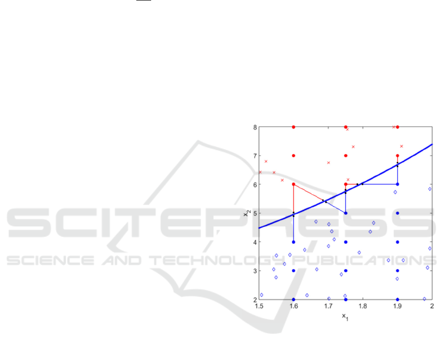
Figure 1: Illustrative example of the methodology to find
the SVM hypersurface points. In red or blue the two
classes (points either of the mesh or the class themselves
and classified according to the SVM). In black the points
found for the hypersurface.
Therefore, for all practical purposes, the points
found as previously described are sufficiently close
to the hypersurface to be considered on it. This way
to obtain SVM hypersurface points for synthetic data
is shown pictorially in Figure 1.
It is good practice to repeat the process also
starting from the other side of the hypersurface, in
order to avoid possible bias in the selection of the
points on the hypersurface. An adequate number of
points is typically a multiple of the support vectors.
One order of magnitudes more points than SVs is a
safe choice, in the sense that all the numerical tests

performed have always provided more than
satisfactory results with this number of points or
higher. If a lower number of points on the
hypesurface are considered, the final equation can be
too smooth and might not fully represent the
complexity of the boundary between the classes.
Attention can also be usefully paid to the fact that the
density of the points reflects the density of the SVs in
the feature space. In any case, it is easy to incraese the
number of points up to the number necessary. The
main limitation here is mainly computational time
(see Section 6) not any principle difficulty.
Once obtained the candidate points sufficiently
near to the hypersurface, before proceeding, it is in
any case good practice to perform some checking.
This can be easily achieved using again the already
trained SVM. It is sufficient to input to the SVM the
candidate points, obtained with the previously
described procedure, and verify that the distance to
the hypersurface is smaller than the error bars.
4.2 How to Derive the Equation of the
Hypersurface via SR
Once it has been verified that sufficient points close
to the hypersurface have been found, the equation of
the hypersurface itself can be estimated using SR via
GP. Indeed the points identified with the procedure
described in the previous subsection are on the
boundary between the two classes. Therefore the
equation of that surface is the equation of the
boundary between the two classes.
An efficient way of retrieving the equation of the
hypersurface from the points consists of regressing
them with SR, using the quantity with the largest
dynamic range as the independent variable. The
quality of the obtained equation can be assessed first
with the statistical indicators described in Section 3.
Moreover, an additional and more conclusive test
can be performed, exploiting again the trained SVM.
In this case, it is indeed possible to generate a series
of points from the candidate formula and insert them
in the SVM. If the distance from these points and the
hypersurface is sufficiently close to zero, it can be
confirmed that indeed the equation is a good
representation of the boundary between the two
classes. As a criterion of closeness to the boundary,
typically the value of the error bars of the
measurements can be taken: if the points generated
by the equation are at a distance from the
hypersurface smaller than the error bars, for all
practical purposes the obtained equation can be
considered a sufficient approximation of the
boundary between the two classes.
5 NUMERICAL TESTS AND
RELATED RESULTS
The procedure described in the previous section has
been subjected to a systematic series of numerical
tests. The results have always been positive and the
proposed technique has always allowed recovering
the original equations describing the boundary
between the two classes. In the following, the
detailed procedures for these numerical tests are
described and some results presented. For clarity’s
sake, mainly low dimensional cases are illustrated in
the following, but it has been verified that the
approach is equally valid for high dimensional cases
(up to 8 or 9 independent variables), provided of
course a sufficient number of examples and adequate
computational resources are available.
5.1 Overall Procedure for Producing
Synthetic Data
The main technique to produce synthetic data and to
test the methodology consists of the following 6
steps:
1- Definition of an initial function for the
boundary;
2- Generating samples of the two classes from
the function
3- Training the SVM for classification
4- Building an appropriate mesh on the domain
5- Determining a sufficient number of points on
the hyper-surface identified by the SVM
6- Deploying SR to identify the equation of the
hypersurface from the points previously
obtained
In the following more details about this
procedure are provided. To fix the ideas, the
discussion is particularized for the case of two
independent variables x
1
and x
2
.
In the first step, an initial function as a
combination of arithmetic, trigonometric, and
exponential operators of independent variables x
i
is
defined. In general, this function can be written as
follows:
=
(
,
,…,
)
∈(
,
)
(8)
In the second step, for the case of two
independent variables, it is typically sufficient to
generate about 4000 random points in the range of
variables for the x
i
and to calculate y for them. Then,

a positive offset and some random values are added
to the y for half of the data to produce the first class;
a negative offset and some random values are added
to y for the other half to produce the second class.
The equations for producing the two classes (
,
)
can be summarized as follow:
=+
(
0,
)
+
=+
(
0,
)
−
(9)
Where c stands for the arbitrary offset and
U(0,L) stands for a random uniform distribution
between 0 and the bulk thickness of data L
Table 1: General GP parameters for the calculation of the
boundary equations.
GP Parameters Value(s)
Population size 500
Selection method Ranking and Tournament
Fitness function AIC
Constant range Integers between -10 and 10
Maximum depth of trees 7
Genetic operators
(Probability)
Crossover (45 %)
Mutation (45 %)
Reproduction (10 %)
In the third step, an SVM with "Gaussian Radial
Basis Function kernel" is trained. The method used
to find the separating hyperplane is "Sequential
Minimal Optimization". Depending on the level of
random noise, different success rates can be
obtained. For the numerical tests presented in the
following, the success rate in the classification of the
SVM is always very close to 100%.
In the fourth step, a mesh on the domain has to
be built in order to identify points sufficiently close
to the hypersurface. For this reason, each dimension
of the domain has been subdivided in one hundred
intervals, producing one million mesh points ( 100
3
).
The fifth step consists of the identification of the
points sufficiently close to the hypersurface, with the
algorithm described in Section 4.
In the sixth step, the selected hypersurface points
are used as inputs to the symbolic regression code,
to find the appropriate formula for describing the
hypersurface. The settings adopted to run the GP
implementing the SR are reported in Table 1.
In the next sections, some examples are provided
to illustrate the applicability and capability of the
presented methodology for systems of increasing
dimensionality and complexity.
5.2 Examples for Two Independent
Variables
As a first test, a quite complex function comprising
exponential, arithmetic, and power operators has
been assumed for the boundary between the two
classes. The function and ranges of the variables are
reported in equation (10):
=
√
⋅
∈
(
0,1
)
,
∈
(
1,3
)
(10)
After carrying out the six-step procedure
previously described, the expression in equation (11)
has been obtained:
= 0.974⋅
√
⋅
(11)
SR via GP converges on a final expression that is
in excellent agreement with the initial function
describing the boundary between the two classes,
even without making recourse to the non-linear
fitting step.
As an additional test, a more complex function
comprising trigonometric and arithmetic operators
has been defined and 4% noise was added to the
database. The function and ranges for the variables
are reported in equation (12):
=sin
(
)
+
∈
(
−3,3
)
,
∈
(
−2,2
)
(12)
After carrying out the six-step procedure
previously described, the expression in equation (13)
has been obtained:
= 0.985
(
sin
(
)
+
)
(13)
Again SR via GP converges on a final expression
that is in excellent agreement with the initial
function describing the boundary between the two
classes, even without making recourse to the non-
linear fitting step. Figure 2 presents the results of
this example in pictorial form.
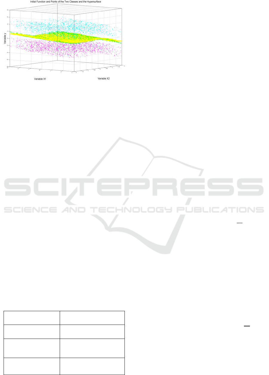
Figure 2: Points and surfaces of the example of equation
(12). Green rectangles are points generated from the initial
function, Cyan points are the points belonging to the first
class, Magenta points are the points belonging to the
second class, and the Yellow surface identifies the hyper-
surface obtained with the SR via GP.
5.3 Effect of Noise and High
Dimensional Data
The numerical examples presented previously
include cases where the success rate of the SVM
classification is close to 100%. This is certainly an
interesting situation from a scientific point of view;
the SVM has learned almost perfectly the boundaries
between the classes and therefore the main issue
remaining consists of formulating the equations of
these boundaries in a mathematical form appropriate
for understanding the phenomena.
On the other hand, it has been checked with
extensive numerical tests that, if the success rate of
classification of the SVM is significantly lower than
100%, the proposed method works well anyway,
since its objective is the reformulation of the
boundary equation found by the SVM. The success
rate required for the SVM and the interpretation of
the results is an issue which depends on the
application and the objectives of the analysis but
does not impact on the validity of the developed
technique.
Table 2: The range of the variables used to generate the
data with function (15).
Steps: Values:
Initial Function Eq.(15)
Ranges of Variables
∈
(
0,2
)
,
∈
(
1.5,3
)
∈
(
−2,4
)
,
∈
(
0,6
)
∈
(
4,12
)
,
∈
(
1,4
)
Number of Nodes for
Each Class
2000
It is worth also emphasizing that the task of SR
in this context is not to improve the success rate of
the SVM classification. The real goal consists of
representing the equations of the boundary between
the classes in more realistic and interpretable
mathematical forms, so that they can be used by the
scientists for actual understanding (for example for
comparison with theories and first principle models).
To achieve this, a reasonable degradation of
classification success rate is tolerable and typically
not a major issue. In any case, with an appropriate
implementation of the proposed method, typically
the performance of SVM can be preserved by the
final equations obtained with symbolic regression.
As mentioned, there is no conceptual difficulty in
applying the proposed methodology to higher
dimensional problems. Of course, the computational
resources required increase exponentially with the
number of independent variables (the so called curse
of dimensionality). Also the number and quality of
the examples must be adequate. But these are
problems related to the available computational
power and/or the quality of the data; in no way they
affect the applicability of the proposed technique.
Indeed it has been verified with a series of
systematic tests that, with adequate level of
computer time, problems in higher dimensions can
also be solved. A quite demanding example is
reported in the following, for an equation involving
7 variables. The equation used to generate the data
is:
=
+
(
)
+
(
)
−
(14)
It is worth mentioning that in many applications
in physic and chemistry one has to deal with
problem of a dimensionality not higher than 7.
Equation (15) is therefore of realistic complexity for
many applications. A total of 4000 points, 2000 per
class, has been generated starting from equation
(14); more details about the synthetic data are
provided in Table 2. After generating the grid,
training the SVM and finding the hyper-surface
points, SR via GP Genetic has been applied and the
expression for the obtained hyper-surface is reported
in equation (15):
= 0.9(
)+sin
(
)
+cos
(
)
−
(15)
The equation found by the method is practically
the original one. The slightly different multiplicative
factor in front is not to be ascribed to a weakness of
the method but to the dataset provided as input,
since the accuracies of both the SVM and the
mathematical equation obtained are equal to 100%.
Again, this example proves that, provided the
surface of the boundary between the cases is
sufficiently regular, the dimensionality is not an
insurmountable issue, if enough computational
power is available.
5.4 Computational Requirements
As an indication about the computational resources
required for the application of the proposed
technique, the run time for an example of 5 variables
has been calculated. Using a computer with 8 cores
and 24 gigabyte of RAM (an Intel Xeon E5520, 2.27
GHz, 2 processors), with Windows 64 bit operating
system, finding the hyper-surface points takes 3
hours and the SR calculation 48 hours. The number
of points on the grid is 16
4
* 51; 16 for the four
independent variables and 51 for the dependent one.
In this respect, the run time to train the SVM is not a
major problem, since it is typically of the order of
minutes and therefore negligible compared to the
other steps of the procedure. Moreover, the
calculation of the grid is also not a major issue since
the step requiring by far most of the computational
resources is the SR. On the other hand, it should be
mentioned that the codes used to obtain these results
had not been parallelized. Therefore, since both the
building of the grid and the Genetic Programs can be
easily parallelized, reduction of the computational
resources of orders of magnitude could be easily
achievable.
6 REAL WORLD EXAMPLES
To show the potential of the proposed methodology
to attack real life problems, in this section its
application to some experimental databases is
reported. The data have been collected in the
framework of various disciplines but the original
measurements have all been obtained via remote
sensing. The term remote sensing indicates the set of
techniques aimed at obtaining information about
objects without being in contact with them. These
techniques can be used to monitor various aspects of
the atmosphere and also the effects of human
activities on the environment.
6.1 Botany: “Wilt” Database
As an example of application to a real-world
problem, first a database related to botany named
“wilt” has been selected. This database was prepared
by Brian Johnson from the Institute of Global
Environmental strategies in Japan in 2013 and
contains the results of a remote sensing study about
detecting diseased trees with Qickbird imagery
(Johnson, 2013). The data set consists of image
parts, generated by segmenting the pansharpened
pictures. The segments contain spectral information
from the Quickbird multispectral image bands and
texture information from the panchromatic (Pan)
image band. In the following, the entries of this
database are listed:
• Class: “w„ (diseased trees) or “n„(all other
land cover)
• GLCM_Pan: GLCM mean texture (Pan
band)
• Mean_G: Mean green value
• Mean_R: Mean red value
• SD_Pan: Standard deviation (Pan band)
This database contains 4339 samples: 74 of them
related to diseased trees and the rest related to all
other land cover. The new proposed methodology
has been applied to this database for finding the
classification hyper-surface between the two
mentioned classes. The entries have been classified
first with the SVM (with the RBF kernel). The
subsequent application of our technique, grid plus
SR, has allowed to find the following equation:
=22.39⋅
(
)
.
(16)
The previous equation provides a Train Accuracy
equals to 99.4% and a Test Accuracy of 99.5 %,
which are practically the same as the SVM, not only
in terms of global statistics but also with regard to
the individual cases properly or improperly
classified. Given the success rate in excess of 99%,
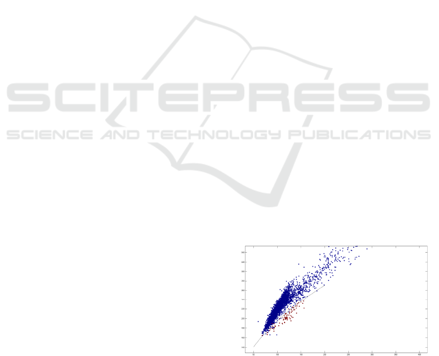
the derived equation (16) indicates that the important
attributes for classifying this database are the Mean
Figure 3: Distribution of data in the “wilt” database. The
red points are diseased trees and the blue points indicate
all other types of land cover. The black line indicates the
equation obtained for the hyper-surface.
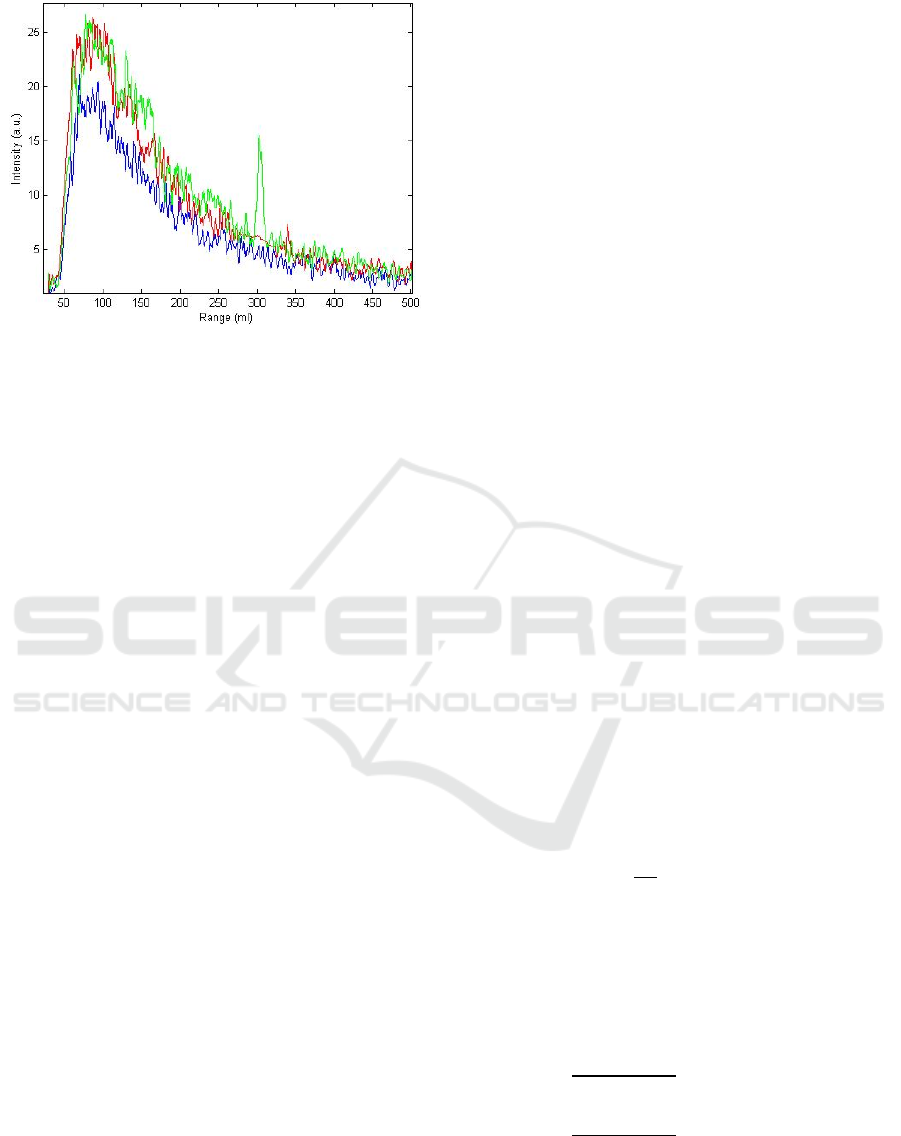
Figure 4: Examples of LIDAR back scattered signals: a)
Clear atmosphere (blue line) b) strong smoke plume
(green line) c) widespread smoke (red line).
green values and the Mean red values. Figure 3
reports the entries of the database projected on the
plane of these two variables, together with the
hyper-surface obtained with equation (16).
It is also worth mentioning that, to obtain the
same success rate, the SVM has to utilize 1299
support vectors. Therefore the application of the
proposed methodology results in a simplification of
orders of magnitude in the complexity of the
equation, without any significant loss in terms of
classification accuracy. Moreover, the obtained
formula is susceptible of comparison with models
and theoretical considerations, whereas the SVM
model is practically intractable from this point of
view. It is worth noting that a metric taking into
account the unbalance in the data, such as positive-
predictive ratio, could in principle be considered,
given the fact that examples of diseased trees are
about two orders of magnitude fewer than the
healthy ones. On the other hand, given the accuracy
already achieved, this would not add much to the
present treatment.
6.2 Remote Sensing of the Atmosphere:
Detection of Widespread Smoke
with LIDAR
One of the remote sensing techniques, which is
gaining increasing importance, is LIDAR an
acronym of Light Detection And Ranging. Lidar
originated in the early 1960s, shortly after the
invention of the laser, and combines laser-focused
imaging with radar's ability to calculate distances by
measuring the time for a signal to return. Its first
deployment was in meteorology and now it is
popularly used as a technology to make high-
resolution maps, with applications in geomatics,
archaeology, geography, geology, geomorphology,
seismology, forestry, remote sensing, atmospheric
physics, laser altimetry and contour mapping.
Wild fires have become a very serious problem
in various parts of the world. The LIDAR technique
has been successfully applied to the detection of the
smoke plume emitted by wild fires, allowing the
reliable survey of large areas (Fiocco, 1963;
Andreucci, 1993; Bellecci, 2007; Bellecci, 2010;
Vega, 2010; Gelfusa, 2014; Gelfusa, 2015).
Recently, mobile compact systems have been
successfully deployed in various environments. Up
to now, the attention has been devoted to early
detection of quite concentrated smoke plumes,
characterizing the first stage of fires, as soon as
possible. The main operational approach consists of
continuously monitoring the area to be surveyed
with a suitable laser and, when a significant peak in
the backscattered signal is detected, an alarm is
triggered. In these applications, the backscattered
signal presents strong peaks, which are detected with
various techniques. In other applications, it would be
interesting also to detect the non concentrated,
widespread smoke, which can be the consequence of
strong wind dispersion or non concentrated sources
(Marrelli, 1998). In this case, the signature of the
presence of the smoke is not a strong peak in the
detected power but an overall increase of large
regions of the curve. Typical examples of
backscattered signals for the alternatives of no
smoke, strong smoke plume and widespread smoke
are shown in Figure 4. Starting from the typical
Lidar equation (Andreucci 1993), it has been
decided to fit the backscattered signal intensity with
a mathematical expression of the form:
=
∙
∙
∙
(17)
where K
1
and K
2
are constants and R is the
range. The data of Figure 4 have been fitted with this
formula. The result of the non linear fit, for the
widespread smoke is reported in equation (18) and
for clear atmosphere in equation (19):
=
2.648∙10
∙
.∙
∙
(18)
=
1.734∙ 10
∙
.∙
∙
(19)
The results of the fit, equations (18) and equation
(19), indicate quite clearly that the parameter K
2
are
very similar for both the case of widespread smoke
and clear atmosphere. On the other hand, there is a
clear difference, of the order of 25% in the constants
K
1
. This is expected since K
1
includes the effect of
the coefficient β, which indeed quantifies the
backscattering properties of the atmosphere
(Andreucci, 1993; Bellecci, 2007; Bellecci, 2010;
Vega, 2010).
Table 3: Main characteristics of the database used for the
LIDAR application.
Total number of data: 521
Number of non-smoke data 312
Number of widespread smoke
data
209
Number of train data (~80%) 431
Number of test data (~20%) 90
Since the attempt to identify the presence of
widespread smoke is a quite pioneering application
of the LIDAR technique, it is important not only to
be able to discriminate between the two situations
but also to provide models for the interpretation of
the physics. In particular, the identification of the
boundary in the space of the parameters K
1
and K
2
for the two cases is considered an essential piece of
information for comparison with theories. The
proposed methodology has therefore been applied to
a quite substantial database summarized in Table 3.
For the SVM, a radial basis functions kernel has
been used. The best equation found is with SR:
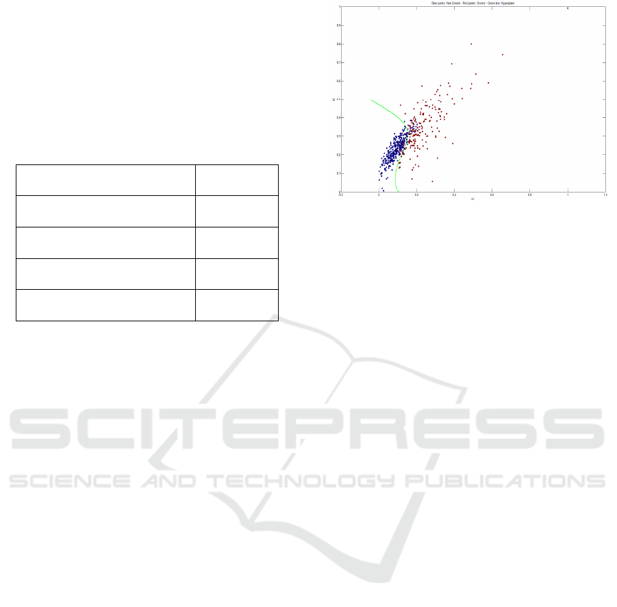
= 0.1083⋅ sin15.61⋅
+
+cos1.59⋅
.
(20)
The above equation provides a Train Accuracy
of 89.33 % and a Test Accuracy of 91.11 %,
practically the same as the SVM success rate. The
equation of the boundary between clear atmosphere
and widespread smoke, in the space of the
parameters K
1
and K
2,
is shown in Figure 5. To
understand the importance of the results obtained, it
should also be considered that the model of the SVM
consists of 154 support vectors. Therefore the level
of simplification obtained with equation (20) is
substantial.
Figure 5: Equation (18), describing the boundary between
the boundary between the cases of clear atmosphere and
widespread smoke, in the space of the parameters K
1
and
K
2
.
7 CONCLUSIONS
An original methodology has been devised to obtain
the equation of the boundary between two classes,
starting from an SVM classifier. In this way, using
SR via GP, the power of machine learning tools is
combined with the realism, physics fidelity and
interpretability of equations expressed in the usual
formalism of typical scientific theories. In particular,
the choice of SVM ensures that their structural
stability, their capability to maximize the safety
margins in the classification, is fully retained in the
final result. On the other hand, symbolic regression
allows finding the best trade-off between accuracy
of the classification and complexity of the final
equations of the boundary, depending on the
application. Moreover, “a priori” information can
also be exploited in order to steer the solutions
towards mathematical expressions, which reflect the
actual dynamics of the phenomena under study. This
can be achieved for example by selecting properly
the basis functions or by constraining the structure
of the trees. Given the fact that the objectives of the
approach are realism and interpretability, a
reasonable reduction of the classification
performance is not a major issue and can be
tolerated. It is also true that symbolic regression via
genetic programming can reproduce the accuracy of
the classification by the SVM, provided a
sufficiently high number of mesh nodes and the
necessary complexity of the SR are allowed for.
The numerical tests shown have proved the
effectiveness of the proposed technique to identify
the real equation of the boundary between classes
even in relatively high dimensions, provided the

shape of the boundary is a sufficiently regular
surface. Again, this seems to be fully adequate since,
in the majority of the scientific applications, the
boundaries between the various classes are quite
regular functions. This has been confirmed by the
application of the technique to experimental
databases of different scientific disciplines.
On the other hand, the method is susceptible of
various improvements. First of all, the technique
should be extended to other machine learning tools,
such a neural networks. More fundamentally, the
approach is now limited to identifying the
mathematical expressions of boundaries which can
be expressed as functions. It is a topic of future
investigations to apply the method to the
investigation of more complex boundaries (for
example multiply connected hypersurfaces).
Moreover, the task of regression, and not only
classification, should also be tackled (Murari (D),
2015; Murari (C), 2015; Peluso, 2014; Murari,
2016). Also applications to various aspects of
tomography inversion and disruptions are envisaged
(Martin, 1997; Murari (B), 2013).
REFERENCES
Andreucci F and Arbolino M., 1993, Il Nuovo Cimento,
16, 1, 35 (1993).
Bellecci C et al, 2007, Appl. Phys. B, 87, 373.
Bellecci C et al., 2010, Optical Engineering, 49 (12),
124302.
Cannas B. et al, 2013, Nucl. Fusion 53 093023
Fiocco G. and Smullin L. D., 1963, Nature, 199, 1275 .
Gaudio et al., 2014, Plasma Phys. Control. Fusion, 56
114002.
Gelfusa M. et al, 2014, Review Scientific Instr., 85,
063112
Gelfusa M. et al, 2015 “First attempts at measuring
widespread smoke with a mobile lidar system”, IEEE
Xplore, ISBN: 978-1-78561-068-4
Hirotugo A., 1974, IEEE Transactions on Automatic
Control 19 (6): 716–723, 1974
Johnson B.et al, 2013, International Journal of Remote
Sensing, 34 (20), 6969-6982.
Kenneth P. B and Anderson D. R., 2002, “Model Selection
and Multi-Model Inference: A Practical Information-
Theoretic Approach”, Springer (2nd ed)
Koza J.R., 1992, “Genetic Programming: On the
Programming of Computers by Means of Natural
Selection”, MIT Press, Cambridge, MA, USA.
Lotov A. V. et al, 2009 “Interactive Decision Maps:
Approximation and Visualization of Pareto Frontier”,
Springer, ISBN 978-1-4020-7631-2.
Marrelli L. et al, 1998, “Total radiation losses and
emissivity profiles in RFX”, Nucl. Fusion 38 (5), 649
Martin P. et al, 1997, Review of scientific instruments 68
(2), 1256-1260
Murari A., et al, 2009, Nucl. Fusion, 49 055028 (11pp)
Murari A., et al. (A), 2013, Nucl. Fusion 53 033006 (9pp)
Murari A., et al, (B), 2013 Nucl. Fusion, 53 043001
doi:10.1088/0029-5515/53/4/043001
Murari A. et al (C), 2015, Plasma Physics. Control.
Fusion, 57 014008, doi: http://dx.doi.org/10.1088/
0741-3335/57/1/014008
Murari A et al (D), 2015, Nucl. Fusion 55 073009 (14pp)
doi:10.1088/0029-5515/55/7/073009
Murari A. et al., 2016, Nucl. Fusion 56 026005,
doi:http://dx.doi.org/10.1088/0029-5515/56/2/026005
Peluso E. et al, 2014, Plasma Phys. Control. Fusion, 56
114001,doi:http://dx.doi.org/10.1088/0741-
3335/56/11/114001
Rattà G. A. et al., 2010, Nucl. Fusion. 50 025005 (10pp).
Schmidt M. and Lipson H., 2009 April, Science, Vol 324
Vapnik V., 2013 “The Nature of Statistical Learning
Theory”, Springer Science & Business Media, ISBN
1475724403, 9781475724400
Vega et al, 2010, Review of Scientific Instruments, 81 (2),
p. 023505
Vega J et al, 2014, Nucl. Fusion 54 123001
Vega J. et al, 2009, Nucl. Fusion. 49 085023 (11pp)
Wesson J., “Tokamaks”, Clarendon Press, Oxford, 2004.
Third edition.
