
Enhanced Symbolic Regression Through Local Variable Transformations
Ji
ˇ
r
´
ı Kubal
´
ık
1
, Erik Derner
1,2
and Robert Babu
ˇ
ska
1,3
1
Czech Institute of Informatics, Robotics, and Cybernetics, Czech Technical University in Prague, Prague, Czech Republic
2
Department of Control Engineering, Faculty of Electrical Engineering, Czech Technical University in Prague,
Prague, Czech Republic
3
Cognitive Robotics, Faculty of 3mE, Delft University of Technology, Delft, The Netherlands
Keywords:
Symbolic Regression, Single Node Genetic Programming, Nonlinear Regression, Data-driven Modeling.
Abstract:
Genetic programming (GP) is a technique widely used in a range of symbolic regression problems, in particular
when there is no prior knowledge about the symbolic function sought. In this paper, we present a GP extension
introducing a new concept of local transformed variables, based on a locally applied affine transformation of
the original variables. This approach facilitates finding accurate parsimonious models. We have evaluated the
proposed extension in the context of the Single Node Genetic Programming (SNGP) algorithm on synthetic as
well as real-problem datasets. The results confirm our hypothesis that the transformed variables significantly
improve the performance of the standard SNGP algorithm.
1 INTRODUCTION
Symbolic regression (SR) is a regression analysis
method formulated as an inductive learning task. The
main principle is to search in a predefined space of
mathematical expressions for a model that fits the
given data as accurately as possible. SR has been
successfully used in nonlinear data-driven model-
ing or data mining, often with quite impressive re-
sults (Schmidt and Lipson, 2009; Vladislavleva et al.,
2013; Staelens et al., 2013; Brauer, 2012). The main
advantage of SR is that it generates parsimonious and
human-understandable models. This is in contrast to
other widely used nature-inspired algorithms, such as
artificial neural networks, which are black box and do
not offer any insight or interpretation of the underly-
ing model.
Symbolic regression is usually solved by means
of genetic programming (GP). On the one hand, this
approach is suitable as there is generally no prior
knowledge on the structure and shape of the sym-
bolic function sought. On the other hand, the search
space in SR is huge so when a pure GP is applied
to a SR task, it needs a long time to find an ac-
ceptable solution. Besides the standard Koza’s tree-
based GP (Koza, 1992), many other variants have
been proposed such as Grammatical Evolution, Gene
Expression Programming, Cartesian GP or Single
Node Genetic Programming. Grammatical Evolution
(Ryan et al., 1998) evolves programs whose syntax
is defined by a user-specified grammar. Gene Ex-
pression Programming (Ferreira, 2001) evolves lin-
ear chromosomes that are expressed as tree struc-
tures through a genotype-phenotype mapping. Carte-
sian GP (CGP) (Miller and Thomson, 2000) uses the
genotype-phenotype mapping to express linear chro-
mosomes as programs in the form of a directed graph.
Single Node Genetic Programming (SNGP) (Jackson,
2012a; Jackson, 2012b) is a GP technique evolving a
population organized as an ordered linear array of in-
terlinked individuals, each representing a single pro-
gram node.
It has been widely reported in the literature that
evolutionary algorithms work much better when hy-
bridized with local search techniques or other means
of final solution optimization. An example is the
memetic algorithm (Hart et al., 2005), where the lo-
cal search is used to fine-tune the candidate solu-
tions along the whole evolution process. A simi-
lar approach can be used to develop efficient GP-
based methods for symbolic regression. Recently,
several evolutionary SR methods emerged that explic-
itly restrict the class of generated models to gener-
alized linear models, i.e., models formed as a lin-
ear combination of non-linear basis functions, also
called features. Examples of these methods are Evo-
lutionary Feature Synthesis (EFS) (Arnaldo et al.,
2015), Multi-Gene Genetic Programming (MGGP)
(Hinchliffe et al., 1996; Searson et al., 2010), Fast
Function Extraction (FFX) (McConaghy, 2011), and
Kubalà k J., Derner E. and BabuÅ ˛aka R.
Enhanced Symbolic Regression Through Local Variable Transformations.
DOI: 10.5220/0006505200910100
In Proceedings of the 9th International Joint Conference on Computational Intelligence (IJCCI 2017), pages 91-100
ISBN: 978-989-758-274-5
Copyright
c
2017 by SCITEPRESS – Science and Technology Publications, Lda. All rights reserved

Single-Run SNGP with LASSO (s-SNGPL) (Kubal
´
ık
et al., 2016). Candidate basis functions are generated
through a standard evolutionary process, while the co-
efficients of the basis functions are found by using a
multiple regression technique. In this way, accurate
linear-in-parameters nonlinear models can efficiently
be evolved.
In this paper, we go one step further towards ro-
bust GP methods for SR. We introduce local trans-
formed variables, which are coordinate transforma-
tions introduced in the individual nonlinear functions.
The motivation for using transformed variables is that
in many cases a good symbolic model is hard to pro-
duce with features in the original coordinate system.
The search process for an acceptable model can be
much more efficient if some of its components use
transformed variables.
We chose a variant of Single Node Genetic Pro-
gramming (Jackson, 2012a; Jackson, 2012b) for a
proof-of-concept implementation of the transformed
variables into GP. It has been shown in (Kubal
´
ık et al.,
2016) that SNGP is good at solving the SR problem.
The concept of transformed variables is general and
can be implemented with other types of GP as well.
In order to facilitate operations with constants, which
is crucial for a proper functioning of the transformed
variables, we used the concept of partitioned popula-
tion, similar to the one introduced in (Alibekov et al.,
2016). The partitioned population is organized so that
it contains a continuous segment of nodes producing
only constant output. These constant-output nodes are
used in and evolved simultaneously with other expres-
sions in the population.
We evaluated the proposed extension on synthetic
as well as real-problem datasets with the number of
dimensions ranging from 2 to 4.
The paper is organized as follows. Section 2 de-
scribes the standard Single Node Genetic Program-
ming algorithm. The novel concept of transformed
variables is introduced in Section 3. Section 4
presents the experiments performed in order to com-
pare the algorithm variants. Finally, the achieved im-
provement of the proposed algorithm extension is dis-
cussed in Section 5.
2 STANDARD SNGP
Single Node Genetic Programming is a graph-based
GP technique that evolves a population organized as
an ordered linear array of individuals, each represent-
ing a single program node. Program nodes can be
of various types depending on the particular problem
solved. In the context of SR the program node can
either be a terminal, i.e. a constant or a variable, or
some operator or function chosen from a set of func-
tions defined for the problem at hand. The individuals
are interconnected in the left-to-right manner, mean-
ing that an individual can act as an input operand
only of those individuals which are positioned to the
right of it in the population. Thus, the whole popu-
lation represents a graph structure similar to that of
the CGP with multiple expressions rooted in individ-
ual nodes. The population is evolved through a first-
improvement local search procedure using a single re-
versible mutation operator.
Formally, the SNGP population is a set M =
{m
0
,m
1
,... ,m
L−1
} of L individuals, with each indi-
vidual m
i
being a single node represented by the tuple
m
i
= he
i
,Succ
i
,Pred
i
,o
i
, f
i
i, where
• e
i
∈ T ∪F is either an element chosen from a func-
tion set F or a terminal set T defined for the prob-
lem;
• Succ
i
is a set of successors of this node, i.e. the
nodes whose output serves as the input to this
node;
• Pred
i
is a set of predecessors of this node, i.e. the
nodes that use this node as an input operand;
• o
i
is a vector of its outputs;
• f
i
is the individual’s fitness.
The population is organized as shown in Figure 1,
starting with constants and variables, followed by
function nodes.
Figure 1: Structure of the standard SNGP population.
Links between the nodes in the population must
satisfy the condition that any function node can use as
its successor (i.e. the operand) only nodes that are po-
sitioned lower down in the population. Similarly, pre-
decessors of individual i must occupy higher positions
in the population. Note that each function node is in
fact a root of an expression that can be constructed by
recursively traversing its successors towards the leaf
terminal nodes.
The fitness of each individual (i.e. of each expres-
sion) is for SR problems typically calculated as the
root mean squared error observed on the set of train-
ing samples.
A simple evolutionary operator called successor
mutation (smut) is used to modify the population. It
picks one individual of the population at random and

then replaces one of its successors by a reference to
another individual chosen among all individuals posi-
tioned to the left of it in the population.
The population is evolved using a local search pro-
cedure. In each iteration, a new population is derived
from the current one by the smut operator. The new
population is then accepted for the next iteration if it
satisfies the chosen acceptance rule (typically, if its
performance is not worse than the performance of the
original population). Otherwise the original popula-
tion remains for the next iteration.
The baseline SNGP implementation used in this
work differs from the one described in (Jackson,
2012a; Jackson, 2012b) in several aspects described
in the following paragraphs.
Form of Regression Models. A hybrid SNGP de-
noted as the Single-Run SNGP with LASSO proposed
in (Kubal
´
ık et al., 2016) is used in this work. It pro-
duces generalized linear regression models. In par-
ticular, candidate features, i.e. expressions rooted in
individual nodes, are combined into generalized lin-
ear regression model using some multiple regression
technique. In this way, precise linear-in-parameters
nonlinear regression models can efficiently be pro-
duced.
Original s-SNGPL uses the Least Absolute
Shrinkage and Selection (LASSO) regression tech-
nique to generate models of limited complexity, i.e.
models composed of a limited number of features. In
particular, all features in the population with a non-
constant output are eligible candidates for the final
model. Though, only some of the candidate features
are used in the final model returned by the LASSO
procedure in the end. An advantage of this LASSO
approach is that a suitable subset of features used in
the model is chosen automatically. On the other hand,
the LASSO procedure is more computationally ex-
pensive than a simple least squares regression. Here,
instead of the LASSO regression operating with large
set of features, we use the simple least squares re-
gression explicitly operating on a fixed number of
features. The complexity of the resulting regression
models is controlled by (i) the maximum depth of fea-
tures evolved in the population, d, and (ii) the maxi-
mum number of features the models can be composed
of, n
f
.
In order to have a possibility to identify the nodes
to be used as features in the linear regression model, a
special type of node called identity node is introduced.
This node has a single successor (i.e. an input), which
is a link to another node in the population. The iden-
tity node then returns outputs of the node it refers
to. The identity nodes are positioned at the end of
the population, see Figure 1. The number of identity
nodes n
i
is equal to the maximum number of features
to be used in the generated models. By changing the
successors of the identity nodes, the set of features for
the generated regression models can be altered. This
is realized in two ways. The first one is by the stan-
dard mutation operator during the evolution. The sec-
ond one is through a local search procedure at line 21
in Algorithm 1. It is launched in the end of each epoch
and runs for a predefined number of iterations, l
i
. In
each iteration, one identity node is randomly chosen
and its successor reference is changed to a new node
randomly chosen from the set of tail partition nodes.
Such a modified population is evaluated, meaning its
linear regression model is constructed using the mod-
ified set of identity nodes (i.e. the features). If the
new model’s fitness is not worse than the fitness of
the original population model, the modification made
to the identity node is accepted. Otherwise, the orig-
inal setting of the identity node remains for the next
iteration.
Fitness. Here, the fitness represents a quality of the
whole generalized linear regression model calculated
as the root mean squared error observed on the set of
training samples. In addition, we also assess a quality
of each single node in the population. This is denoted
as the node’s utility and it is calculated as the Pearson
product-moment correlation coefficient between the
node’s output and the desired output over the set of
training samples.
paragraphSelection Strategy. In the original
SNGP, nodes to be mutated are selected purely at ran-
dom. Here we use a variant of tournament selection
(see line 12 in Algorithm 1). It operates with util-
ity values assigned to the nodes during the population
evaluation step at line 3 and 15, respectively. When
selecting the node to be mutated, t candidate individ-
uals are randomly picked from the population at first.
Then, out of the candidates the one that is involved
in the best-performing expression with respect to the
root node utility value is chosen. In this way, not only
nodes that have high utility values themselves are be-
ing favoured. Instead, all nodes at least contributing
to high-quality expressions are preferred to the ones
not playing an important role in the population (i.e.
the nodes not involved in any well-performing expres-
sion).
Evolutionary Model. The process of evolving the
population is carried out in epochs. In each epoch,
multiple independent parallel threads are run for a
predefined number of generations, all of them start-
ing from the same population, which is the best final

population out of the previous epoch threads. This re-
duces the chance of getting stuck in a local optimum.
The model is parameterized by the number of threads
n
t
, the epoch length l
e
, and the number of epochs n
e
.
3 PROPOSED EXTENSIONS
In this section, we describe the concept of trans-
formed variables, introduced in order to make the
SNGP algorithm more efficient at solving the SR
problem.
3.1 Transformed Variables
The transformed variables are obtained by local affine
transformations of the coordinate system. Assume n-
dimensional input space X ⊂ R
n
. Each transformed
variable v is represented by the tuple
v = hw
0
,c
0
,x
0
,. .. ,w
n
,c
n
,x
n
i
where c
j
is a pointer to a constant-valued node in the
population, w
j
∈ R is a real-valued constant, x
j
is the
jth original variable, with x
0
= 1 corresponding to
the offset of the transformation. The constant-valued
nodes referred to by the c
j
pointers are either basic
constant nodes (i.e. nodes from the first section of the
partitioned population in Figure 2) or head partition
nodes. The value of the transformed variable v is cal-
culated as
v =
n
∑
j=0
b
j
x
j
,
where b
j
= w
j
o
j
with o
j
the output of the node refer-
enced by c
j
. The weighting coefficients are formed as
b
j
= w
j
o
j
in order to allow for both global and local
tuning of their values. In particular, changing the ref-
erence c
j
to a different constant-valued node is likely
to lead to a significant change of the corresponding
b
j
. On the contrary, fine-tuning of the coefficient b
j
can be achieved by applying small changes to w
j
. The
values of w
j
are initialized to 1. The links c
j
are tuned
by means of the standard mutation operator.
Both c
j
and w
j
can further be tuned through a lo-
cal search procedure, see line 22 in Algorithm 1. It
is launched in the end of each epoch and runs for
a predefined number of iterations, l
v
. In each itera-
tion, one transformed variable v
k
is randomly chosen
and either its reference to the constant-valued node c
k
or the value of w
k
is changed with equal probability.
The value of w
k
is modified by adding a random value
drawn from a normal distribution as follows:
w
k
= w
k
+ N(0,1).
The population with the modified node v
k
is evalu-
ated and if its fitness is not worse than the fitness of
the original population, the modification made to the
node v
k
is accepted. Otherwise, the original setting
of the transformed variable node remains for the next
iteration.
3.2 Partitioned Population
To support the concept of transformed variables, the
population is organized so that the function nodes
are further divided into two continuous segments, the
head and tail partitions as introduced in (Alibekov
et al., 2016). The head partition nodes are allowed
to represent root nodes of expressions producing only
constant output. The tail nodes can be roots of both
the constant-output as well as variable-output expres-
sions. The head partition therefore represents a pool
of constants that are used in and evolved simultane-
ously with other features in the population.
The number of transformed variables n
v
and the
number of head partition nodes n
h
are user-defined
parameters. Note that besides the transformed vari-
ables the population always contains also all the orig-
inal variables x ∈ {x
1
,. .. ,x
n
}. The structure of the
partitioned population is shown in Figure 2.
Figure 2: Structure of partitioned population.
3.3 Algorithm SNGP-TV
The whole algorithm, denoted here as SNGP with
transformed variables (SNGP-TV), is outlined in Al-
gorithm 1. It iteratively evolves current best popula-
tion of individuals P and the corresponding model M.
The main loop, lines 5–29, iterates through epochs.
In each epoch, multiple independent threads are run,
lines 7–24, all of them started with the same popula-
tion P, line 8. Each thread runs for a predefined num-
ber of generations, lines 11–20. In the end of each
thread, the identity nodes and transformed variables
are tuned for a specified number of trials, lines 21–
22. The best final population and its model are saved
in P and M, lines 25–27, and P becomes the starting
population for next epoch. Finally, the last version of
model M is returned as the solution.

Algorithm 1: SNGP with transformed vari-
ables.
Input: training data set, L, n
c
, n
h
, n, n
v
, n
f
, d,
l
i
, l
v
, l
e
, n
e
, n
t
1 initialize population P
2 build regression model M using P
3 evaluate M
4 e ← 0
5 do
6 t ← 0
7 do
8 P
t
← P
9 M
t
← M
10 generation ← 0
11 do
12 s ← selectNode(P
t
)
13 P
0
t
← mutate(P
t
,s)
14 build model M
0
t
using P
0
t
15 evaluate M
0
t
16 if (M
0
t
is not worse than M
t
)
17 P
t
← P
0
t
18 M
t
← M
0
t
19 generation ← generation +1
20 while (generation < l
e
)
21 [P
t
,M
t
] ← optIdentityNodes(P
t
,l
i
)
22 [P
t
,M
t
] ← optTrans fVars(P
t
,l
v
)
23 t ← t + 1
24 while (t < n
t
)
25 b ← argbest
t=1,...,n
t
(M
t
)
26 P ← P
b
27 M ← M
b
28 e ← e +1
29 while (e < n
e
)
30 return M
Output: symbolic model M
4 EXPERIMENTS
4.1 Test Datasets
For the proof-of-concept experiments we used thir-
teen datasets, featuring both synthetic and real data,
with the number of dimensions ranging from 2 to
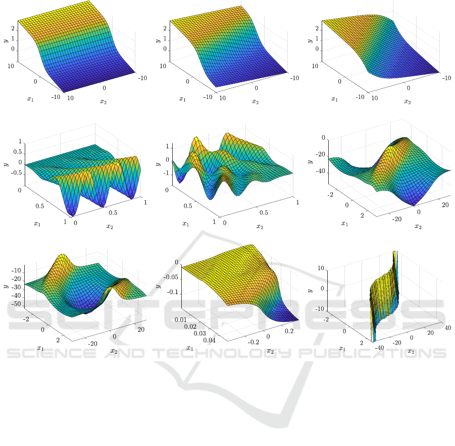
4. Figure 3 shows mesh plots of all 2-dimensional
datasets used.
To demonstrate how the transformed variables fa-
cilitate finding models of functions in a transformed
space, we used the synthetic datasets sig0, sigπ/8
and sigπ/4 shown in Figures 3(a) through 3(c). The
dataset sig0 was calculated using a sigmoid-like func-
tion, defined by Equation 1, sampled on a regular grid
of 31 × 31 points for x
1
,x
2
∈ [−10,10].
f
1
(x) = 0.1x
1
+
2
1 + e
−x
1
(1)
Note that x
2
is not used in the equation and there-
fore, the values of the function do not change along
the x
2
dimension. The function was then rotated by
π/8 rad (dataset sigπ/8) and π/4 rad (dataset sigπ/4)
in the counterclockwise direction in order to simulate
the transformation of the coordinate system.
Other two synthetic datasets f2 and f3 (Figures
3(d) and 3(e)) were generated using the following
functions:
f
2
(x) = x
2
1
cos(10x
1
− 15x
2
), (2)
f
3
(x) =(x
1
− 1)
2
cos(10(x
1
− 1) − 15(x
2
− 1)) (3)
−(x
2
− 1)
2
sin(10(x
1
− 1) + 15(x
2
− 1)),
sampled on a regular grid of 31 × 31 points in the in-
terval x
1
,x
2
∈ [0,1].
The following datasets come from the domain of
reinforcement learning applications.
The 1dof dir dataset (Figure 3(f)) consists of sam-
ples of the value function approximator for a 1-DOF
inverted pendulum swingup (Adam et al., 2012). The
pendulum moves in a state space defined by variables
α ∈ [−π, π],
˙
α ∈ [−40, 40], where α denotes the an-
gle and
˙
α is the angular velocity of the pendulum.
The pendulum is pointing up for α = 0. The 961 data
points were sampled on a regular grid with 31 samples
in each dimension. The 1dof inv dataset (Figure 3(g))
is a variant of the 1-DOF swingup problem, which
differs in the interpretation of the angle α. The pen-
dulum is pointing down for α = 0, whereas both for
α = −π and α = π, the pendulum is pointing up.
The magman dataset (Figure 3(h)) is based on a
magnetic manipulation (Hur
´
ak and Zem
´
anek, 2012)
problem. The magnetic manipulation setup consists
of two electromagnets in a line positioned at a = 0 m
and a = 0.025 m. The dataset is represented by sam-
ples of the value function approximator on the domain
x
1
∈ [0,0.05], x
2
∈ [−0.4,0.4], where x
1
= a is the po-
sition and x
2
= ˙a is the velocity. The data are sampled
on a regular grid of 31 × 31 points.
The policy dataset represents samples of the pol-
icy function for the direct inverted pendulum task,
described above. The policy function was sampled
on the range x
1
∈ [−π,π], x
2
∈ [−40,40]. From the
whole state space, only the samples in the transition
region were used and the plateaus were removed from
the dataset, see Figure 3(i). In order to retain the num-
ber of training data points comparable with the rest of
the datasets used in the experiments, these data were

sampled on a regular grid with a higher resolution of
61 × 61 points. The policy dataset comprises 313 data
points.
The last dataset related to the reinforcement learn-
ing, denoted 2dof, is derived from the value function
for an inverted pendulum with two links. It is a 4-
dimensional problem with the angle α
i
and angular
velocity
˙
α
i
describing the state of each link i ∈ {1,2}.
The dataset consists of 6561 data points sampled on
a regular grid with nine samples evenly distributed in
each dimension.
4.2 Experiment Setup
We experimentally evaluated the proposed SNGP-TV
algorithm and compared it to two other variants of
SNGP – namely the SNGP with simple population
(see Figure 1) denoted as SNGP-SP and the SNGP
with partitioned population (see Figure 2) but not us-
ing the transformed variables, denoted as SNGP-PP.
Note, both the variants can be described by the Algo-
rithm 1 if the population type and control parameters
are set accordingly. The SNGP-SP and SNGP-PP dif-
fer in the population type while none of them uses
the transformed variables, so n
v
= 0 and l
v
= 0. The
SNGP-TV was tested with the number of transformed
variables being equal to the number of the original
variables, i.e. n
v
= n.
Other control parameters were set as follows:
• population size: L = 500
• total number of fitness evaluations: 20.000
• epochs: n
e
= 20, n
t
= 2
• trivial constants: C = {0,0.5,1,2,3,4}, n
c
= 6
• original variables: n = 2
• maximum tree depth: d = 7
• basic functions:
F
1
= {∗,+,−,square,cube,BentIdentity
1
},
F
2
= {∗,+,−,square,cube,Sigmoid}
• maximum number of features: n
1
f
= 10, n
2
f
= 3
• SNGP-SP: l
e
= 650, l
i
= 150
• SNGP-PP: l
e
= 650, l
i
= 150, n
h
= 121
• SNGP-TV: l
e
= 500, l
i
= 150, l
v
= 150, n
h
= 120
We carried out three experiment series:
1. experiment-1 – all compared algorithms were run
on all datasets with function set F
1
and the maxi-
mum number of features n
1
f
= 10.
1
Bent identity is a non-linear, unbounded, monotonic
function that approximates identity near the origin, see
http://www.wow.com/wiki/Activation function.
2. experiment-2 – all compared algorithms were run
on all datasets with function set F
1
and the maxi-
mum number of features n
2
f
= 3.
3. experiment-3 – algorithms SNGP-PP and SNGP-
TV were run on synthetic datasets sigπ0, sigπ/8,
and sigπ/4 with function set F
2
and the maximum
number of features n
2
f
= 3.
The first two experiments were run to support our hy-
pothesis that the use of the transformed variables in
GP can be beneficial. The two experiments differ
in the complexity of the evolved general regression
models. Our hypothesis is that when more complex
models (in terms of the maximum number of evolved
features combined in the linear regression models) are
allowed, then even less effective algorithms (i.e. the
ones not using the transformed variables) can be able
to construct a good model. On the other hand, when
less complex models are allowed, the advantage of us-
ing the transformed variables should prove more sig-
nificant. Experiment-3 is proposed to illustrate that
when the population contains some feature or its part
that might well describe the data if its input was prop-
erly transformed, then this can efficiently be achieved
with the transformed variables. In this case the key
element of the model sought is the sigmoid function
that was added to the set of basic functions in place of
the BentIdentity function.
Each experiment was replicated 30 times with the
root mean squared error (RMSE) calculated for each
single run. The median RMSE over the 30 runs is
used as the performance measure in the tables with
results. The Wilcoxon rank sum test (also known as
the Mann-Whitney U-test) was used to evaluate sta-
tistical significance of the difference in performance
between two algorithms.
Besides the RMSE, the complexity of the pro-
duced models was analyzed as well. In general, the
complexity of a model was calculated as the total
number of nodes in the model. More precisely, the
model complexity equals the sum of the complexi-
ties of the features that the model is composed of,
plus the operators and weights that are used to join
the features into one expression (the whole regres-
sion model). The following assumptions were made
for the calculation of a complexity of the SNGP-PP
and SNGP-TV models. In the case of SNGP-PP and
SNGP-TV, each constant-valued tree rooted in a head
partition node was treated as a single constant-valued
node. Thus, if some tail partition function node takes
a head partition node as its input, then this head par-
tition node is counted as a single node, even though
it is effectively represented by a more complex tree
structure. The rationale behind this assumption is that
the head partition was introduced into the population
(a) (b) (c)
(d) (e) (f)
(g) (h) (i)
Figure 3: Mesh plots of the datasets. The intersections of the grid represent the data used as the input for the SNGP algorithm
and its variants. The following datasets were used in the experiments: from (a) to (c) – synthetic sigmoid-like function
described by Equation 1, rotated by (a) 0 rad, (b) π/8 rad and (c) π/4 rad; (d), (e) – synthetic functions described by Equation
2 and 3, respectively; (f), (g) – variants of inverted pendulum, (h) – magnetic manipulation; (i) – policy function for inverted
pendulum (transition region only).
in order to facilitate a production of constant-valued
expressions that act as single constants in the final
models. Similarly, each transformed variable node in
SNGP-TV is treated as a single variable node, even
though it is effectively represented by a more com-
plex structure, see Section 3.1.
Note, we restrict our experiments to compare only
the SNGP variants – SNGP with and without the
transformed variables. We do not include any other
GP method into the analysis since we simply want
to demonstrate that if the transformed variables are
used in some GP method for solving the symbolic re-
gression problem, then it leads to an improved perfor-
mance of that method. We did not tune control param-
eters of the compared SNGP algorithms either since
the purpose of the experiments was not to present
the best possible performance of the algorithms on
the test data sets. Again, we just wanted to show
the difference between using and not using the trans-
formed variables with the other control parameters set
the same for both variants. It is very likely that if we
tuned the control parameters of the SNGP, the perfor-
mance of the compared variants, both the one with
and the one without the transformed variables, would
improve.
4.3 Results
Results for experiment-1 are summarized in Table 1,
Table 2 and Table 3. Table 1 presents the median
RMSE values. Table 2 shows which algorithms out-
perform the other algorithms. A given algorithm out-
performs another algorithm on a given dataset if both
of the following two conditions are met:

Table 1: Medians of RMSE for all tested algorithms and
datasets in experiment-1.
Dataset
SNGP variant
Scale
SP PP TV
sig0 8.75 8.51 6.98 ×10
−4
sigπ/8 5.42 5.45 0.46 ×10
−2
sigπ/4 1.64 2.85 0.26 ×10
−2
f2 2.76 2.64 1.59 ×10
−1
f3 4.06 4.00 3.26 ×10
−1
1dof dir 2.82 2.82 1.34 ×10
0
1dof inv 2.50 2.20 2.22 ×10
0
magman 8.54 7.51 3.55 ×10
−3
policy 1.88 1.88 1.84 ×10
0
2dof 5.24 5.24 4.66 ×10
1
Table 2: Comparison of performance of algorithms in
experiment-1. The table shows which algorithms are out-
performed by the algorithm in the column heading for each
dataset. The performance is compared using the Wilcoxon
rank sum test with a significance level of 1 %. The entry
with an asterisk would be included if the significance level
was increased to 5 %.
Dataset
SNGP variant
SP PP TV
sig0
sigπ/8 SP, PP
sigπ/4 SP, PP
f2 SP, PP
f3 SP, PP
1dof dir SP, PP
1dof inv SP SP
magman SP SP, PP
policy SP, PP*
2dof SP, PP
• its RMSE median is smaller than the RMSE me-
dian of the compared algorithm,
• the Wilcoxon rank sum test rejects the null hy-
pothesis that the RMS errors in the 30 runs for
each of the two algorithms are samples from dis-
tributions with equal medians, at the statistical
significance level of 1 % and 5 %, respectively.
In the case of 1 % significance level, the null hypothe-
sis for the pair of SNGP-PP and SNGP-TV algorithms
was not rejected on 3 datasets. When the signifi-
cance level was increased to 5 %, the null hypothesis
was not rejected on 2 datasets. Table 3 presents the
median complexity of models produced by the three
compared variants. It shows that the complexity of
SNGP-TV models, as defined in Section 4.2, is in
most cases less than the complexity of the SNGP-SP
and SNGP-PP models.
Table 3: Medians of complexity for all tested algorithms
and datasets in experiment-1.
Dataset
SNGP variant
SP PP TV
sig0 108 106 100
sigπ/8 119 121 104
sigπ/4 119 117 102
f2 137 144 125
f3 128 133 119
1dof dir 122 122 106
1dof inv 126 119 112
magman 132 144 122
policy 118 118 119
2dof 103 106 106
Table 4: Medians of RMSE obtained with SNGP-PP and
SNGP-TV in experiment-2.
Dataset
SNGP variant
Scale
PP TV
sig0
4.07 2.41
×10
−2
sigπ/8
1.43 0.72
×10
−1
sigπ/4
1.45 0.42
×10
−1
f2
2.98 2.74
×10
−1
f3
4.31 4.17
×10
−1
1dof dir
5.20 4.03
×10
0
1dof inv
5.00 4.31
×10
0
magman
1.04 0.73
×10
−2
policy
3.21 2.92
×10
0
2dof
8.40 7.01
×10
1
Results for the experiment-2 are summarized in
Table 4. Here, the null hypothesis was rejected at the
1 % significance level for all datasets with the excep-
tion for the policy dataset. When the significance level
was increased to 5 %, the null hypothesis was rejected
for all datasets. Thus, the improvement provided
by the transformed variables is even more significant
when smaller models are evolved as demonstrated by
the increased number of datasets on which SNGP-TV
proved to be significantly better than SNGP-PP com-
pared to the results observed in experiment-1. Simi-
larly as in the experiment-1, the complexity of SNGP-
TV models is in most cases less than the complexity
of the SNGP-PP models, see Table 5.
Results for the experiment-3 are summarized in
Table 6. Both SNGP-PP and SNGP-TV variants per-
form equally well on the unrotated dataset sig0 as the
null hypothesis was rejected neither at the 1 % nor 5 %
significance level. This is in accordance with our ex-
pectation that this dataset is easy for the algorithms
since they only need to generate and combine sim-
ple linear and sigmoid features with a single input x
1
.

Table 5: Medians of complexity obtained with SNGP-PP
and SNGP-TV in experiment-2.
Dataset
SNGP variant
PP TV
sig0
32 32
sigπ/8
32 37
sigπ/4
37 35
f2
57 47
f3
49 49
1dof dir
40 36
1dof inv
40 35
magman
53 42
policy
41 39
2dof
39 38
Table 6: Medians of RMSE obtained with SNGP-PP and
SNGP-TV in experiment-3.
Dataset
SNGP variant
Scale
PP TV
sig0
6.26 6.75
×10
−10
sigπ/8
9.61 0.17
×10
−2
sigπ/4
3.72 0.13
×10
−2
Table 7: Medians of complexity obtained with SNGP-PP
and SNGP-TV in experiment-3.
Dataset
SNGP variant
PP TV
sig0
24 22
sigπ/8
38 25
sigπ/4
33 29
On dataset sigπ/4, a significant difference in perfor-
mance between SNGP-PP and SNGP-TV can already
be observed. However, even SNGP-PP was able to
find a solution with RMSE lower than 6.5 × 10
−10
in
10 out of 30 runs. These results correspond to models
that employ a sigmoid feature with a simple argument
(x
1
+x
2
). A similar trend of SNGP-TV outperforming
SNGP-PP was observed on the sigπ/8 dataset where
SNGP-TV achieves by more than one order of mag-
nitude better RMSE than SNGP-PP. Moreover, the
best solution obtained with SNGP-PP had an RMSE
of 7.7 × 10
−5
, while SNGP-TV generated five solu-
tions with RMSE lower than 6.5 × 10
−10
. Again,
the complexity of SNGP-TV models is lower than
the complexity of the SNGP-PP models, see Table 7.
The most significant difference being observed on the
sigπ/8 dataset, which is the one with the most ”diffi-
cult” transformation of the input space.
5 CONCLUSIONS
The concept of local transformed variables for sym-
bolic regression was introduced, so that the genetic
programming search for an accurate model is more ef-
ficient. We have integrated transformed variables into
the Single Node Genetic Programming algorithm, us-
ing a partitioned population with certain nodes ex-
plicitly devoted to producing constant-output expres-
sions.
The experimental results show that the proposed
SNGP with transformed variables outperforms the
baseline SNGP algorithm on the majority of test
datasets. We found that the transformed variables
are especially useful when parsimonious models are
sought.
Our future research will focus on incorporating
model complexity control into the algorithm, which
may further boost the performance of the approach.
ACKNOWLEDGMENT
This research was supported by the Grant Agency
of the Czech Republic (GA
ˇ
CR) with the grant
no. 15-22731S titled “Symbolic Regression for Re-
inforcement Learning in Continuous Spaces” and
by the European Regional Development Fund un-
der the project Robotics 4 Industry 4.0 (reg. no.
CZ.02.1.01/0.0/0.0/15 003/0000470).
REFERENCES
Adam, S., Bus¸oniu, L., and Babu
ˇ
ska, R. (2012). Experi-
ence replay for real-time reinforcement learning con-
trol. IEEE Transactions on Systems, Man, and Cyber-
netics. Part C: Applications and Reviews, 42(2):201–
212.
Alibekov, E., Kubal
´
ık, J., and Babu
ˇ
ska, R. (2016). Sym-
bolic method for deriving policy in reinforcement
learning. In Proceedings of the 55th IEEE Conference
on Decision and Control (CDC), pages 2789–2795,
Las Vegas, USA.
Arnaldo, I., O’Reilly, U.-M., and Veeramachaneni, K.
(2015). Building predictive models via feature syn-
thesis. In Proceedings of the 2015 Annual Conference
on Genetic and Evolutionary Computation, GECCO
’15, pages 983–990, New York, NY, USA. ACM.
Brauer, C. (2012). Using Eureqa in a Stock Day-Trading
Application. Cypress Point Technologies, LLC.
Ferreira, C. (2001). Gene expression programming: a new
adaptive algorithm for solving problems. Complex
Systems, 13(2):87–129.

Hart, W. E., Smith, J. E., and Natalio, K. (2005). Recent
Advances in Memetic Algorithms. Springer, Berlin,
Heidelberg.
Hinchliffe, M., Hiden, H., McKay, B., Willis, M., Tham,
M., and Barton, G. (1996). Modelling chemical pro-
cess systems using a multi-gene genetic programming
algorithm. In Koza, J. R., editor, Late Breaking Papers
at the Genetic Programming 1996 Conference Stan-
ford University July 28-31, 1996, pages 56–65, Stan-
ford University, CA, USA. Stanford Bookstore.
Hur
´
ak, Z. and Zem
´
anek, J. (2012). Feedback lineariza-
tion approach to distributed feedback manipulation. In
American control conference, pages 991–996, Mon-
treal, Canada.
Jackson, D. (2012a). A new, node-focused model for ge-
netic programming. In Moraglio, A., Silva, S., Kraw-
iec, K., Machado, P., and Cotta, C., editors, Genetic
Programming: 15th European Conference, EuroGP
2012, M
´
alaga, Spain, April 11-13, 2012. Proceedings,
pages 49–60. Springer, Berlin, Heidelberg.
Jackson, D. (2012b). Single node genetic programming
on problems with side effects. In Coello, C. A. C.,
Cutello, V., Deb, K., Forrest, S., Nicosia, G., and
Pavone, M., editors, Parallel Problem Solving from
Nature - PPSN XII: 12th International Conference,
Taormina, Italy, September 1-5, 2012, Proceedings,
Part I, pages 327–336. Springer, Berlin, Heidelberg.
Koza, J. R. (1992). Genetic Programming: On the Pro-
gramming of Computers by Means of Natural Selec-
tion (Complex Adaptive Systems). MIT Press Ltd.
Kubal
´
ık, J., Alibekov, E.,
ˇ
Zegklitz, J., and Babu
ˇ
ska, R.
(2016). Hybrid single node genetic programming for
symbolic regression. In Nguyen, N. T., Kowalczyk,
R., and Filipe, J., editors, Transactions on Compu-
tational Collective Intelligence XXIV, pages 61–82.
Springer, Berlin, Heidelberg.
McConaghy, T. (2011). FFX: Fast, scalable, determin-
istic symbolic regression technology. In Riolo, R.,
Vladislavleva, E., and Moore, J. H., editors, Genetic
Programming Theory and Practice IX, pages 235–
260. Springer New York, New York, NY.
Miller, J. F. and Thomson, P. (2000). Cartesian genetic pro-
gramming. In Poli, R., Banzhaf, W., Langdon, W. B.,
Miller, J., Nordin, P., and Fogarty, T. C., editors, Ge-
netic Programming: European Conference, EuroGP
2000, Edinburgh, Scotland, UK, April 15-16, 2000.
Proceedings, pages 121–132. Springer, Berlin, Hei-
delberg.
Ryan, C., Collins, J., and Neill, M. O. (1998). Gram-
matical evolution: Evolving programs for an arbi-
trary language. In Banzhaf, W., Poli, R., Schoenauer,
M., and Fogarty, T. C., editors, Genetic Program-
ming: First European Workshop, EuroGP’98 Paris,
France, April 14–15, 1998 Proceedings, pages 83–96.
Springer, Berlin, Heidelberg.
Schmidt, M. and Lipson, H. (2009). Distilling free-
form natural laws from experimental data. Science,
324(5923):81–85.
Searson, D. P., Leahy, D. E., and Willis, M. J. (2010). GP-
TIPS : An open source genetic programming toolbox
for multigene symbolic regression. In Proceedings
of the International Multiconference of Engineers and
Computer Scientists 2010 (IMECS 2010), volume 1,
pages 77–80, Hong Kong.
Staelens, N., Deschrijver, D., Vladislavleva, E., Vermeulen,
B., Dhaene, T., and Demeester, P. (2013). Construct-
ing a no-reference H.264/AVC bitstream-based video
quality metric using genetic programming-based sym-
bolic regression. IEEE Transactions on Circuits and
Systems for Video Technology, 23(8):1322–1333.
Vladislavleva, E., Friedrich, T., Neumann, F., and Wagner,
M. (2013). Predicting the energy output of wind farms
based on weather data: Important variables and their
correlation. Renewable Energy, 50:236–243.
