Deep Associative Semantic Neural Graphs for Knowledge

Representation and Fast Data Exploration

Adrian Horzyk

Department of Automatics and Biomedical Engineering, AGH University of Science and Technology in Krakow,

Mickiewicza Av. 30, 30-059 Krakow, Poland

Keywords: Active Knowledge-based Neural Structures, Semantic Neural Structures, Representation of Complex Entities,

Knowledge-based Inference, Deep Neural Network Architectures, Associative Graph Data Structures, Big

Data, Associative Database Normalization, Database Transformation, Data Mining, Knowledge Exploration.

Abstract: This paper presents new deep associative neural networks that can semantically associate any data, represent

their complex relations of various kinds, and be used for fast information search, data mining, and knowledge

exploration. They allow to store various horizontal and vertical relations between data and significantly

broaden and accelerate various search operations. Many relations which must be searched in the relational

databases are immediately available using the presented associative data model based on a new special kind

of associative spiking neurons and sensors used for the construction of these networks. The inference

operations are also performed using the reactive abilities of these spiking neurons. The paper describes the

transformation of any relational database to this kind of networks. All related data and their combinations

representing various objects are contextually connected with different strengths reproducing various

similarities, proximities, successions, orders, inclusions, rarities, or frequencies of these data. The

computational complexity of the described operations is usually constant and less than operations used in the

databases. The theory is illustrated by a few examples and used for inference on this kind of neural networks.

1 INTRODUCTION

Efficient and safe collecting, storage, retrieval,

processing, mining, and exploration of big data are

the most important tasks of contemporary computer

science (Apiletti et al., 2017), (Han and Kamber,

2000), (Piatetsky-Shapiro and Frawley, 1991),

(Fayyad, 1996), (Jin et al., 2015), (Linoff and Berry,

2011), (Pääkkönen and Pakkala, 2015). To get

benefits from various big data collections, we need to

use smart and very fast methods for data search,

mining, and knowledge exploration. It is not an easy

task because data are typically stored in relational

databases which relate data and entities only

horizontally. Data must be sorted, indexed, or joined,

and vertical relations must often be found and

processed in many time-consuming nested loops.

This paper introduces new deep associative

semantic neuronal graphs (DASNG) which allow for

storing data where the data are automatically

horizontally and vertically associated and ordered

according to all attributes without any substantial

computational or memory costs. Moreover, these

relations can be easily supplemented by any further

relations or related objects that can be added to this

structure or stored in a result of data exploration using

extra neurons and connections. Vertical data

associations describe many useful relations like

similarity, proximity, order, or succession in space or

time. They can also easily determine minima,

maxima, medians, average numbers, and data ranges.

Data mining and knowledge exploration methods

usually try to find interesting groups of similar,

different, frequent, or infrequent patterns for a given

minimum support and minimum confidence to define

associative rules, cluster objects or draw some useful

conclusions about objects or their groups (Agrawal et

al., 1993), (Apiletti et al., 2017). The introduced

model of the data representation and storage in the

DASNG structure supplies us with an ability to

directly or indirectly connect related data. This

strategy excludes computationally expensive loops

and reduces the computational complexity of

operations on the related data. All minima and

maxima are available in constant time. All other

values of each attribute are organized using the

Horzyk A.

Deep Associative Semantic Neural Graphs for Knowledge Representation and Fast Data Exploration.

DOI: 10.5220/0006504100670079

In Proceedings of the 9th International Joint Conference on Knowledge Discovery, Knowledge Engineering and Knowledge Management (KEOD 2017), pages 67-79

ISBN: 978-989-758-272-1

introduced aggregated values B-trees which

automatically aggregate and count duplicated values

and order them linearly during their construction

process. This strategy reduces the computational

complexity of many operations.

The introduced DASNGs consist of a special kind

of spiking neurons introduced in this paper and

referring to the earlier models presented in (Horzyk,

2014), (Horzyk et al., 2016), (Horzyk, 2017). Spiking

neurons are reactive and use a time approach for

computations (Gerstner and Kistler, 2002), so data

exploration routines can be triggered in these graphs

automatically by stimulation of neurons representing

any search context. It is very useful because some

frequently performed operations are built-in this

neural system and do not need to be implemented in

the form of typical algorithmic procedures. The

connection network between neurons allows us to

quickly find associated data, objects, and patterns

accordingly to their frequency, similarity, or vicinity

in raw data. Furthermore, all important findings can

be almost costless converted into new neuronal

substructures that will store them in the same graph

for any further use and inference.

The way, in which the DASNGs work, classify

them as emergent cognitive neuronal systems. They

have a few similar features to semantic networks and

other emergent cognitive systems (Duch and Dobosz,

2011), (Nuxoll and Laird, 2004), (Parisia et al., 2017),

(Starzyk, 2007), (Starzyk, 2015). The semantic

networks represent semantic relations between

concepts that are linked together (Sowa, 1991), while

in the introduced DASNGs, neurons can represent

any sets of elementary or complex sub-combinations

of input data and directly or indirectly related objects

for defining differing contexts affecting the neurons

with different strength. Semantic networks are

browsed through using various search routines

operating on graph structures, while the presented

associative graphs are equipped with special reactive

spiking neurons that can automatically perform some

search operations by stimulating them. It will be

shown how neurons process such search operations

and how this neural graph works on exemplary data

in section 6.

2 RELATIONAL DATABASE

MODEL DRAWBACKS

In computer science, we used to store data in

relational databases, consisting of tables, which use

primary and foreign keys to represent related entities.

In relational databases, we use entity-relational model

(ER model) that describes interrelated things of

interest in a specific domain of knowledge (Bagui and

Earp, 2011), (Chen, 2002). The above-mentioned ER

model is composed of entity types which classify the

things of interests and specifies various horizontal

relationships that can exist between instances of those

entity types. This model is also an abstract data model

that defines a data structure that can be implemented

as a relational database. The ER modeling was

developed for database design by Peter Chen (Chen,

2002). However, the ER model can also be used in the

specification of domain-specific ontologies.

Entities may be characterized not only by

relationships but also by additional properties

(attributes), which include special identifies called

primary keys. In the databases, each row of a table

represents one instance of an entity type, and each

field represents an attribute type, where a relationship

between entities is implemented by storing a primary

key of one entity as foreign keys in other entities of

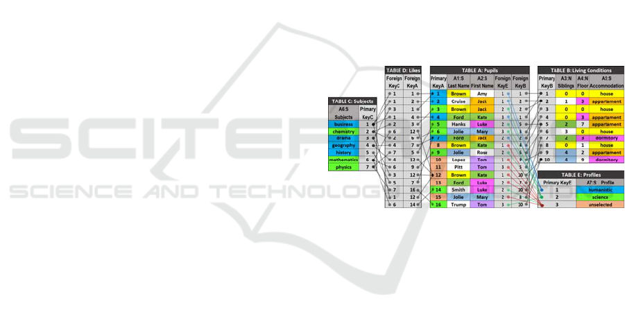
other tables (Fig. 1).

Figure 1: A sample of the small database with typically

repeated attribute values and relations to the same objects

of another table represented by the primary keys.

In the relational database model, features are

grouped in rows defining entities (records, tuples,

objects) collected in tables. The rows of different

tables can be horizontally linked together using

primary and foreign keys. This kind of row linking

allows defining more complex objects by other

already represented objects in other tables. Keys are

unique, sorted, and usually quite quickly available

using B-trees, B+trees, hash-tables, or other methods

typically in logarithmic time (Cormen et al., 2001),

(Hellerstein et al., 2007).

All modern databases use a Cost Based

Optimization (CBO) to optimize queries and to create

and an individual execution plan for each query.

Usually, there are many possibilities, which

dependently on row numbers and created indices can

differ computational cost and complexity of various

execution plans. Execution plans can comprise

dynamically created temporal indices for the current

query if it improves the cost of the execution plan.

Many times, heuristic or greedy algorithms are also

used to quickly find out a “good” enough execution

plan without brute force search (Hellerstein et al.,

2007).

Moreover, we distinguish various join operations

as nested loop join, hash join, and merge join which

can be more efficient in some specific situations. The

join operations are frequently executed on every

database, so their optimization is crucial. The nested

loop join takes O(N*M) time, the hash join is

processed in O(N+M) time, and the merge join in

O(N+M) or O(N*log N + M*log M) dependently on

working on the sorted or unsorted data, where N and

M are the numbers of merged records of two joined

tables (Hellerstein et al., 2007).

Statistics are also very useful and help to estimate

the disk I/O and CPU operations and memory usage

to find a “good” enough execution plan, however,

there is a certain cost of updating statistics as well.

The I/O disk data access for reading and writing

operations are bottlenecks of databases, especially

when a database is huge and do not fit into memory

because disk operations are typically at least hundreds

of times slower than operations executed in the RAM.

Despite the many advantages of such a solution,

we also come across many difficulties and

bottlenecks, where the ER data model is not effective

enough (Hellerstein et al., 2007), e.g. the time

necessary to update statistics and indices, sorting

operations, cope with hundred times slower I/O disk

operations, quick finding a good enough execution

plan for each query, or the necessity to frequently

search for various vertical relations between entities

of the same table. One of the main drawbacks of the

relational database model, which is addressed in this

paper, is in the limited way of binding data and

objects vertically. Vertical relations between entities

and their defining values stored in columns are not

represented (Fig. 1). This lack forces database

management systems (DBMS) to search for vertical

relations in many loops using SQL operations if the

information about such relations is required. The SQL

search operations (SELECT) in relational databases

are typically the most frequent operations, so

inefficiency of them costs a lot of time which is most

annoying and very expensive when managing huge

data collections.

Moreover, the objects can be naturally ordered

only after a single selected attribute in each table. If it

is necessary to have data sorted after several attributes

simultaneously, indices must be used. The indices

typically use B+trees or hash tables to sort and

organize data to make them available in logarithmic

time. The main drawbacks of using indices are the

relevant additional memory cost and the slowdown of

addition, updating, and removal operations. In result,

it is not recommended to add indices for data

attributes which data are not frequently used in search

operations. This paper presents how to overcome

these drawbacks and organize data in such a way that

both horizontal and vertical relations are represented

in the proposed associative neuronal graph data

structure described in the following sections.

3 AVB-TREES

In this section, a new self-ordering and self-balancing

tree structure is proposed to efficiently organize input

elements of the further introduced associative neural

structures and get a very fast access to all stored

features and objects. This structure, called AVB-tree

(Aggregated-Values B-tree), is similar to the well-

known B-tree structure, but it automatically

aggregates and counts all duplicates (Fig. 2). Thus,

the AVB-trees store only unique values of each

attribute defining stored objects. Despite the

aggregation of duplicates, this operation does not

diminish the information about the stored objects.

The neurons representing these unique attribute

values can have many connections to neurons

representing objects. Hence, AVB-trees are usually

much smaller than B-trees or B+trees constructed for

the same data, where duplicates are not aggregated.

The aggregation of the same values also saves the

memory and accelerates the access to the stored

objects, especially to the related objects which are on

the top of interests and usually searched by queries.

The counting of duplicates makes possible to remove

data from this structure correctly.

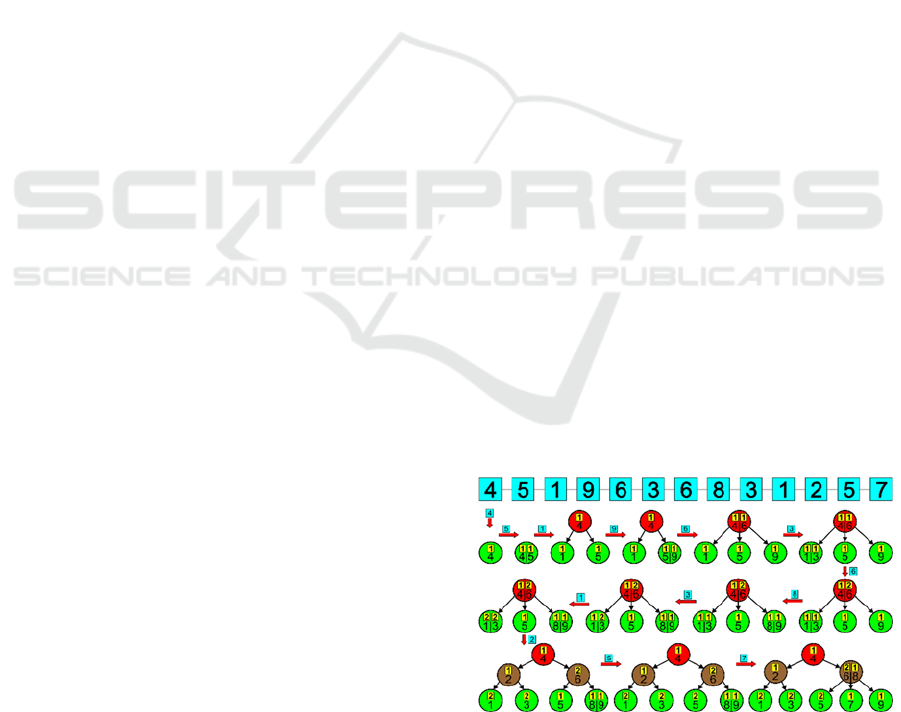
Figure 2: Construction of an exemplary AVB-tree.

The AVB-trees are constructed in a very similar

way as the B-trees, however, several important chan-

ges must be implemented in it:

The insertion of the next key to the AVB-tree is

processed as follows (Fig. 3):

1. Start from the root and go recursively down along

the edges to the descendants until the leaf is not

achieved after the following rules:

 if one of the keys stored in the node equals to

the inserted key, increment the counter of this

key, and finish this operation,

 else go to the left child node if the inserted key

is less than the leftmost key in the node,

 else go to the right child node if the inserted

key is greater than the rightmost key in the

node,

 else go to the middle child node.

2. When the leaf is achieved:

 and if the inserted key is equal to one of the

keys in this leaf, increment the counter of this

key, and finish this operation,

 else insert the inserted key to the keys stored

in this leaf in the increasing order, initialize its

counter to one, and go to step 3.

3. If the number of all keys stored in this leaf is

greater than two, divide this leaf into two leaves

in the following way:

 let the divided leaf represent the leftmost

(least) key together with its counter;

 create a new leaf and let it to represent the

rightmost (greatest) key together with its

counter;

 and the middle key together with its counter

and the pointer to the new leaf representing the

rightmost key pass to the parent node if it

exists, and go to step 4;

 if the parent node does not exist, create it (a

new root of the AVB-tree) and let it represent

this middle key together with its counter, and

create new edges to the divided leaf

representing the leftmost key and to the leaf

pointed by the passed pointer to the new leaf

representing the rightmost key (Fig. 2). Next,

finish this operation.

4. Insert the passed key together with its counter to

the key(s) stored in this node in the increasing

order after the following rules:

 if the key comes from the left branch, insert it

on the left side of the key(s);

 if the key comes from the right branch, insert

it on the right side of the key(s);

 if the key comes from the middle branch,

insert it between the existing keys.

5. Create a new edge to the new leaf or node pointed

by the passed pointer and insert this pointer to the

child list of pointers immediately after the pointer

representing the edge to the divided leaf or node.

6. If the number of all keys stored in this node is

greater than two, divide this node into two nodes

in the following way:

 let the existing node represent the leftmost

(least) key together with its counter;



create a new node and let it represent the

rightmost (greatest) key together with its

counter;

 the middle key together with its counter and

the pointer to the new node representing the

rightmost key pass to the parent node if it

exists and go back to step 4 (Fig. 2);

 if the parent node does not exist, create it (a

new root of the AVB tree) and let it represent

this middle key together with its counter, and

create new edges to the divided node

representing the leftmost key and to the node

pointed by the passed pointer to the new node

representing the rightmost key (Fig. 2). Next,

finish this operation.

The removal of the key from the AVB-tree is

processed very similarly as for B-trees with respect to

the counters of individual keys that must be gradually

decreased to zero for each removed object before

removing a given countered key from this structure.

During this operation, the AVB-tree is self-balanced

in the same way as is proceeded for B-trees (Cormen

et al., 2001).

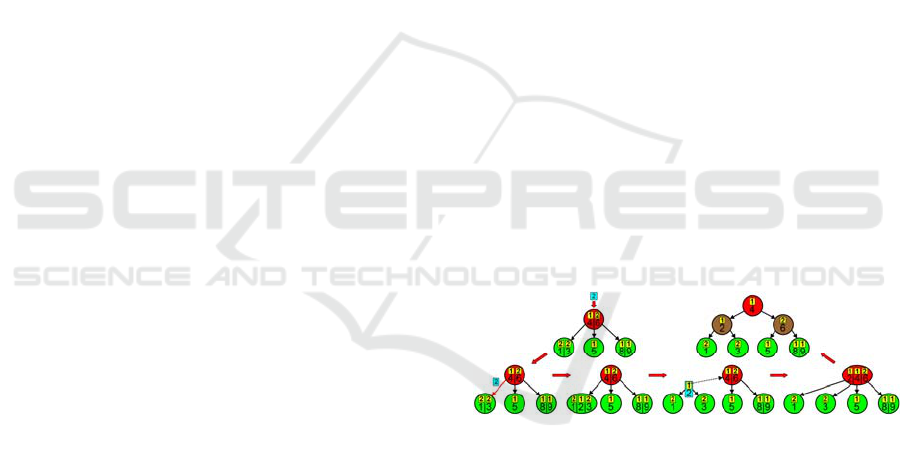
Figure 3: The intermediate steps of passing the middle key

to the parent node after the division of a leaf or a node.

The search operation in the AVB-tree is

processed as follows:

1. Start from the root and go recursively down along

the edges to the descendants until the searched key

or the leaf is not achieved after the following

rules:

 If one of the keys stored in the node equals to

the searched key, return the pointer to this key.

 else go to the left child node if the searched

key is less than the leftmost key in this node.

 else go to the right child node if the searched

key is greater than the rightmost key in this

node.

 else go to the middle child node.

2. If the leaf is achieved and no stored key in it

equals the searched key, return the null pointer.

The search operation for any key in the above-

introduced AVB-trees is very efficient because the

maximum number of search steps is equal to the

logarithm of the number unique keys stored in them,

i.e. 















, where 





is the number of the

unique keys of the attribute 



. Considering that the

attribute values are typically many times repeated in

the database table rows, the number of all entities 

in the table is usually much bigger than the number of

unique values 





of each attribute 



(≫





Hence, the logarithm computed for the usually

constant number of unique values 





for AVB-trees

is usually smaller than the logarithm of the number of

all entities (rows)  used in the search operations

using B-trees or B+trees in relational databases, i.e.





























≅





. The

computational complexity of the insertion, removal,

and update operations in AVB-trees is the same as for

the search operation. It is typically constant

independently of the size of data tables thanks to the

aggregation property of AVB-trees.

Each key element in the AVB-tree structure

represents a sensor which is most sensitive to the

value represented by the key. The sensors stimulate

connected value neurons which can be connected to

any number of object neurons representing objects.

4 SENSORS AND ASSOCIATIVE

SPIKING NEURONS

The presented associative neural graph structures in

the next section will use special kinds of sensors and

associative spiking neurons (ASN), which enable fast

inference using various combinations of stimuli of the

network elements. These graphs consist mainly of

numerical and symbolic sensors, value neurons, and

object neurons to represent tabular data.

In these associative neural graphs, all non-key

database table attributes 



,…,



are transformed

into sensory input fields 





,…,





and all attribute

values are represented by sensors 







,…,







which

are organized using the introduced AVB-trees.

Sensors aggregate all duplicates of each attribute 



separately. Each sensor 







represents all duplicates

of the value 







, so for large data collections, we

usually achieve high memory savings without any

loss of information. It is possible because each value









represented by the sensor 







and subsequently

by a connected value neuron 







can be repeatedly

connected to various object neurons that represents

various entities which contains this value. While

attribute values can define entities in database tables,

here sensors together with value neurons representing

values can define object neurons representing entities.

Each sensor 







is connected to a value neuron









which is stimulated by this sensor with a constant

stimulus 









computed after:























1





























0









































0

(1)

Value neurons 







and 







representing numerical

neighbor values 







and 







of the same attribute 



are additionally mutually connected, and their

weights are computed after the formula:



,







,





1

























(2)

where 





















is the range of all already

represented values of the attribute 



, and 







and









are the minimum and maximum values of this

attribute appropriately. The range is automatically

updated by each sensory input field 





when a new

minimum 







or maximum 







is introduced.

Each numerical attribute 



is additionally

equipped with special extreme sensors 







and









sensitive for existing and new minima and

maxima. These sensors compute their output values

using the following formulas:





































0















1





0

(3)





































0















1





0

(4)

The output values of sensors define the strength of

stimulation of the connected extreme neurons 







and 







which continuously stimulated achieve their

spiking thresholds after the certain periods of time:































0

∞







0

(5)



























0

∞







0

(6)

The extreme sensor 







or 







stimulate the

extreme neurons 







and 







with strength equal

to one only if the current minimum or maximum

value is presented on the 





. The stimulation 















is stronger than one only if there is presented a

new minimum or maximum value which causes the

achievement of the spiking threshold of the 















neuron in time 







1 or 







1. Such a

strong stimulation of the extreme neuron starts a

conditional plasticity routine that brakes the existing

connection from extreme neuron 







or 







to the

connected value neuron 







, and a new connection to

the new created value neuron representing a new

extreme value is established, and its weight is set to

one. It updates the minimum value 







or maximum

value 







and range 





appropriately. In other

cases, the extreme sensors stimulate the connected

neurons with strength less than one, so the neurons

fire later (5) or (6) according to the distance of the

presented value to the extreme ones.

Each sensor 







is connected to its value neuron









which is stimulated and charged by this sensor

as long as the input value 





is presented on the

sensory input field 





. All value neurons used for

the associative transformation of databases into the

DASNG neuronal systems have their activation

thresholds equal to one (







1). According to this

fact, each stimulated value neuron 







solely by its

connected sensor 







achieves its spiking threshold









after the time 









calculated after:









































































1





























0

∞ 





















(7)

In the next step of the associative transformation,

there are created object neurons 







,…,







for each

table 



that does not contain foreign keys. These

neurons represent entities, so they are connected to

the adequate value neurons representing attribute

values which define these entities. The weights of the

connections from these value neurons to the object

neurons should reproduce rarity of the values

represented by value neurons in the defining various

object neurons, so they are defined as the reciprocal

of the numbers of all connections that come from the

given value neuron 







to all connected object

neurons 







representing the entities of the table 





,













:



















(8)

These weights can be easily updated when a new

entity is added, or an existing one is removed. These

weights do not even need to be stored in a neural

network structure because they can be locally and

very fast calculated before each neuronal spike.

Next, there are created object neurons 







for the

tables 



which contain not only attributes but also

some foreign keys for which the object neurons 







representing primary keys have been already created

in the previous steps. The connection weights that

come from the object neurons 







representing

primary keys to the object neurons 







containing

adequate foreign keys are computed as the reciprocal

of the numbers of connections that comes from the

given object neurons 







to all connected object

neurons 







representing the entities of the table 





,









:



















(9)

The weights (8) and (9) allow for the stimulation of

the postsynaptic object neurons with the strength

reflecting the rarity of the values or the entities

represented by the presynaptic neurons. It means that

frequent values and entities have a smaller impact on

the postsynaptic object neurons, while rare values and

entities have a bigger impact and can faster charge

postsynaptic neurons to their spiking thresholds. Each

unique value and entity which primary key is used

only once as a foreign key in another table

(representing the relation 1:1) have the biggest

possible impact because its connection weight is

equal to one, and such a connection can solely charge

the postsynaptic object neuron to its spiking

threshold. The interpretation is quite intuitive because

such features or entities exclusively identify objects

that should also be automatically recognized in any

natural or artificial cognitive neural system.

The spiking threshold of each object neuron must

be achieved ultimately when all defining inputs start

to charge it. However, it can be achieved earlier when

any sub-combination of enough rare inputs happens.

All defining inputs of each object neuron can achieve

the following maximum strength of stimulation:













,









,











(10)

The object neuron’s spiking threshold is defined as:













1









0





















0

(11)

The associative spiking neurons used for modeling of

the value and objects neurons incorporate the concept

of time and implement charging, discharging,

relaxation, and absolute and relative refraction

processes (Fig. 4) (Kalat, 2012). They can also be in

resting state when not stimulated for a longer time.

All internal neuronal processes are modeled using

linear functions that can be easily added, subtracted,

or combined for charging, discharging, or

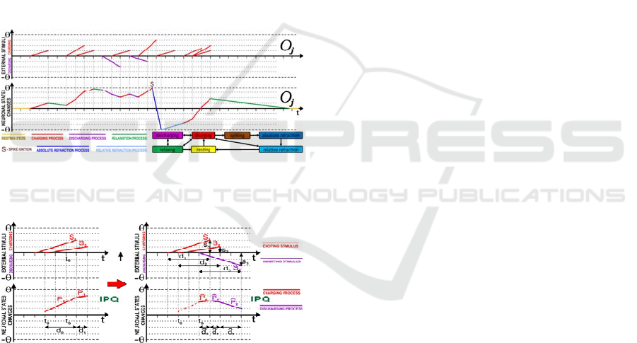
overlapping stimuli (Fig. 4). All external stimuli

influence on internal neuronal processes which

change states of neurons (Fig. 4-5).

Figure 4: Overlapping charging and discharging external

stimuli influencing the state changes and internal neuronal

processes of associative spiking neurons.

Figure 5: The illustration of the operation that combines the

new stimulus S

with the processes P

and P

in the IPQ

created for previous stimuli S

and S

where d

determines

the duration of the stimulus S

, and s

is its strength.

The ASNs work parallel and combine the external

input stimuli that can appear at any time. To simulate

them on a sequential CPU, they use an internal

process queue (IPQ) to manage and switch internal

processes P

and update neuronal states at the right

time (Fig. 5), and a global event queue (GEQ) to order

and execute these internal processes of all neurons at

an appropriate moment and sequence. The GEQ

watches out the time when processes finish to start

updating neurons at the right time. The expected

moments of achievement of spiking thresholds (11)

of individual neurons are always calculated in

advance and watched out. Different than in the

artificial neural networks of the second generation

(Haykin, 2009), which answers are produced by

various values of the output neurons, ASN answers

are produced based on their frequencies of spikes and

the elapsed time from a given external stimulation

moment to the moments when these neurons start

spiking. Hence, the most frequently spiking neurons

represent the answer that can be read from connected

neurons representing the associated objects and

values.

5 DASNG - DEEP ASSOCIATIVE

SEMANTIC NEURAL GRAPHS

Brains consist of many complex and very deep graph

structures of connected neurons of various kinds

(Longstaff, 2011), which use thousands of

connections to represent our knowledge and make our

intelligence work smartly, quickly, and context-

sensitively (Kalat, 2012).

In this section, new deep associative semantic

neural graphs (DASNG) will be introduced to

demonstrate how relational databases can be

transformed into these graphs. Figure 6 illustrates a

neuronal DASNG structure that represents all data

and their relations from the sample database

presented in Fig. 1. This neuronal structure does not

reduce any information so that it can always be

transformed back into the original database. The

DASNG can be constructed for any database storing

related records. In any formal database or cognitive

model, we can distinguish individual data which are

related in different ways. Some groups of related data

model objects (represented by e.g. entities) that can

also be related between themselves in various ways

(e.g. using primary and foreign keys), which describe

semantic relations between them. Such relations can

reproduce similarity, proximity, inclusion, sequence,

actions etc. Such relations can group objects and

define their classes based on similar features. Such

kinds of tasks should be solved in computational

intelligence and knowledge engineering because our

intelligence is based on the ability to discover various

relations and find interesting groups among other

things. To find such relations, the algorithms use

various conditions, limitations, search routines, and

operations which compare or group objects to satisfy

defined requirements or achieve given goals.

The introduced DASNG model can naturally

reproduce data, entities, and all relations that are

represented by the primary-foreign key relational

model. Classes of objects can be defined based on the

similarity between objects which some subsets of

attribute values are the same or close. In the DASNG

model, all the same values are aggregated and all

similar attribute values are directly or indirectly

connected. Consequently, all related objects are fast

accessible thanks to these aggregations and

connections between neurons representing similar

values. The similarity between objects can be

defined as any subset of close attribute values

(features) that relates the group of objects. Thus, all

possible clusters coming from similarity are naturally

included in the DASNG model. In consequence, any

class of objects can be quickly found in the DASNG

network because the stimulation of a subgroup of

sensors representing selected features will gradually

induce activation of connected neurons representing

objects (entities) which the most meet the given

limitations defined by these features as will be

described in the following section.

The DASNG model can also represent other

relations that usually come from object vicinity in

time or space. Vicinity can be defined as an attribute

of time or space where the two compared objects

occur in the close time interval, or their coordinates

are not too far away. Therefore, the vicinity is a

distance in space or time in which objects can interact

with each other or can be perceived as being

neighboring or subsequent by somebody. Close

objects in space or time cannot be similar at all, so we

do not include vicinity as an attribute that groups

objects into classes, but we talk about object

neighborhood or succession. Thus, vicinity can relate

objects independently of their similarity or

differences. Therefore, we can define any sequence of

objects or actions, and elaborate various procedures

and algorithms that come from our intelligence and

knowledge about objects, their features, and

usefulness. Moreover, not only directly subsequent

objects but also more distant ones in any sequence or

neighborhood can be connected and these

connections appropriately weighted to emphasize the

right contexts of their occurrences which exclude

ambiguity. This feature is very important in view of

storing various complex sequences, procedures, or

algorithms that can be applied only in some specific

situations, contexts, constraints, or circumstances, in

which our brains make us undertake a specific

strategy or action selected from the portfolio of the

possible ones that are available to us.

In the DASNG model, objects represented by

neurons are connected to other neurons that represent

other objects or specific features. Each connection is

appropriately weighted to reproduce the strength of

the similarity, vicinity, or defining relations between

them. In comparison to the non-weighted primary-

foreign key binding mechanism used in databases, we

achieve more precise information about the relation

strengths of related objects when representing them in

the DASNG model, so we can conclude about the

represented relations easier and more accurately.

Summarizing, the DASNG model enriches the

horizontal relations used in the databases with

additional vertical relations between objects thanks to

aggregations of the same values and connections

between neighbor values. The use of reactive sensors

and neurons instead of passive database records

allows for fast automatic exploration of information

according to the context given by the stimulation of

any selected subset of sensors and/or neurons.

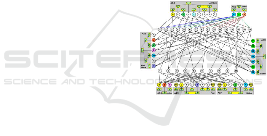
Figure 6: A deep associative semantic neural graph

(DASNG) constructed for the database presented in Fig. 1

without any loss of information, where first letters represent

appropriate words from the database tables.

In the relational database model, we can

distinguish one-to-one, one-to-many, and many-to-

many relationships between related entities. The one-

to-many relationship is represented by a primary key

in one entity (e.g. in table E in Fig. 1) which is related

to many foreign keys of other entities (e.g. in table A

in Fig. 1). The many-to-many relationship defines

multiple relations between various objects from two

tables, so we typically use an additional link table

which binds together primary keys of these tables

(e.g. the table D relates entities of the tables A and C

in Fig. 1). The link tables are unnecessary in the

DASNG networks because we can directly represent

many-to-many relations using direct connections

between objects represented by neurons (Fig. 6). This

is also true for one-to-many relations where objects

are directly connected in the same way. Hence, we do

not need to distinguish between various cardinalities

of relations as in relational databases.

Each attribute is represented by a separate sensory

input field 





which consists of sensors representing

aggregated attribute values, i.e. various features of

objects. All sensors of each field 





are organized

using a separate AVB-tree (Fig. 2). Such a structure

makes all values quickly available, usually in

constant time, however, the sub-linearithmic access

time may also happen for rarely frequent features.

Moreover, numerical value neurons connect in order,

so there is no need to sort data later (Fig. 2).

In the relational databases, modeled objects are

stored in separate or connected table entities

(records), while in the DASNG model, each object

can be represented by a single neuron connected to

other neurons defining features and included objects

in it. If more than one database record contains the

same set of attribute values and foreign keys, these

records can be aggregated and represented by the

same object neuron that counts the number of

aggregated records. This aggregation does not

eliminate diversity because the aggregating neuron

can be further connected to various other neurons

representing differing features for various aggregated

objects. However, during such an aggregation, we

lose the unique identity of the aggregated objects

represented by the primary keys that diversify such

records, e.g. two people with the same first and last

name. When the diversity of records (objects) is

necessary, the primary key must be treated as an

attribute feature that cannot be reduced in the

aggregation process. In result, such objects will not

be aggregated and do not lose their identity and

separateness fixed by their primary keys. On the other

hand, the aggregation is many times beneficial, and

we do not need to store the separate identities of all

objects, e.g. it is usually unimportant to store the

information about which exact entities of the same

products have been sold by which the seller. It is

possible to automatically distinguish between tables

that represent objects that cannot lose their identity

and other tables where we can do aggregations. The

primary keys that are directly used by SQL queries to

search for records are non-reducible and should be

treated as other attributes that store important data.

On the other hand, when the primary keys are used

only to join records from the related tables, such keys

are reducible and can be converted to connections

between neurons. Hence, we need to analyze a

possibly large subset of real SQL queries that have

been processed on the given database in the past to

automatically and correctly distinguish between

reducible and non-reducible primary keys. In case,

when we get a collection of empirical data records,

where some records are identical (e.g. a few samples

in the Iris data set from ML Repository), they can also

be aggregated and represented by the same neurons.

Concluding, aggregations are very important in view

of generalization, knowledge formation, and drawing

conclusions about objects, so we should not always

trend to store identities of all objects if not necessary.

Another benefit of direct connections between

neurons representing objects is that we do not need to

browse primary and foreign keys to join records from

various tables and waste time. In the DASNG

network, we simply go along the connections to

associated information in constant time.

Figure 7: Various kinds of sensory stimuli and interactions

with sensors in the sensory input fields (SIFs).

During the construction process, there is created a

sensory input field 





for each attribute 



(the grey

fields in Figs. 6, 8-10). The sensory input fields (SIFs)

can be of various types alike the senses in a human

body. These fields constitute input interfaces for the

remaining part of the neural structure (Fig. 6). The

SIFs contain sensors that are sensitive for some

values, their ranges, or subsets (Fig. 7). The sensors

can be differently sensitive to various values

presented to their SIF. They are no sensitive to the

values presented to the other SIFs. The way the

sensors work can be described by suitable

mathematical functions introduced in section 4.

The structure presented in Fig. 6 represents not

only horizontal relations between objects but also

vertical relations between data of each attribute.

These data are ordered, and all duplicated values of

each attribute are removed. Despite this reduction,

there is no loss of information because the duplicated

values have been replaced by connections to various

neurons representing various objects in Fig. 1.

Moreover, the aggregation of duplicates and their

joined representation allow for very fast access to any

data. Databases use B-trees or B+trees to achieve a

logarithmic time of search operations while DASNGs

use AVB-trees which for a constant set of stored

unique attribute values usually work in constant time.

Hence, we also do not waste so much time during

insertion or delete operations like when using indexes

in databases. We do not need to sort data or add

indices to this structure because data are always

automatically sorted simultaneously for all attributes.

Furthermore, the transformation of the table structure

to the presented graph structure automatically

extracts additional relations of their order, similarity,

minima, maxima, ranges from the data, which are

available on demand in constant time. Thanks to the

aggregation and joined representation of duplicates

we have direct access to all objects (records) that have

some given value which we want to explore. We also

have indirect but very fast access to all similar objects

which are defined by similar attribute values. Thus,

we can also define various clusters of similar objects

or recognize their defined classes represented by

neurons very fast for any criteria. The stimulation of

any subset of features, their ranges, or any subset of

objects induces gradual activations of the associated

objects neurons, which can be clustered on this basis.

The object class can be retrieved based on the first or

most frequently activated class neuron. Every such

stimulation of DASNG takes constant time, so it is

fast in comparison to many other methods.

The use of ASNs in the DASNG network makes

possible to develop a reactive graph structure that can

execute some operations on the represented data fully

automatically. Such operations let us draw useful

conclusions about objects and their features

represented in this neural network.

6 NEURONAL INFERENCE

After the transformation of the database tables into

the DASNG neural network presented in Fig. 6, this

network can be used for inference about represented

objects to find similar objects quickly, various classes

of objects, identify shared features, filter or sort

objects after various criteria, attributes, or draw some

useful conclusions about selected groups of objects.

Figures 8, 9, and 10 present exemplary inference

processes that can be performed in this DASNG

network. To filter out objects including some features

or other objects, it is enough to stimulate these

features or objects via sensors or neurons representing

them in the DASNG network and wait for spikes of

neurons representing answers (Fig. 8). In such a

network, it works like associative reminding in a

human brain when recalled information together with

the previous calling context create a new context for

recalling of the next memories associated with the

information represented by the recently activated

neurons. Therefore, the further stimulation of the

initial context (here: the sensor representing

“science”) induce the gradual activations of the next

connected neurons representing associated

information about previously recalled objects (Fig.

9). Thus, we can automatically find out what are the

names of pupils who like science, what subjects they

like at most, and what are their living conditions. We

can conclude about them as far as the created

structure contains such information and as long as the

sensor “science” is stimulated providing subsequent

spikes of the directly or indirectly connected neurons.

If the network works parallel, then we always get all

this information in constant time.

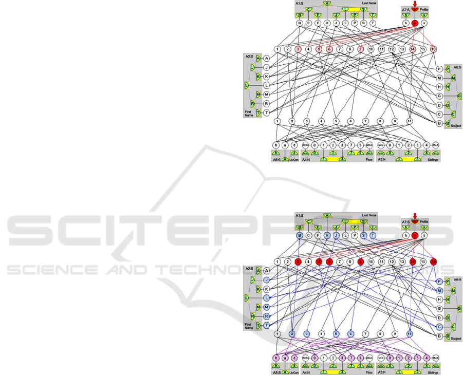
Figure 8: Direct connections from the stimulated value

neuron representing “science” let us quickly filter out pupils

who are interested in science.

Figure 9: The next stimulation lets us find out what subjects

do these pupils like and what are their living conditions.

The inference processes in the DASNG neural

network are based on measuring the time when the

ASN neurons representing the desirable answer(s)

start spiking and on counting the numbers of their

spikes (Fig. 10). Neurons representing the answer

spike most frequently and typically start to spike at

first. The less frequently or later spiking neurons

usually represent other weaker alternatives, i.e.

objects that only partially satisfy the input conditions

or the associated features of the objects representing

the answer. On this basis, we can conclude that pupils

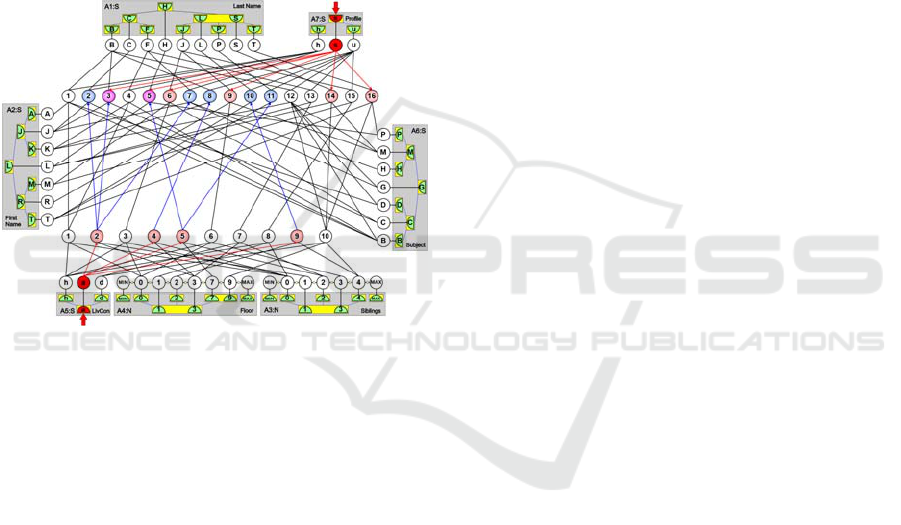
represented by the most frequently spiking neurons 3

(Jack Brown) and 5 (Luke Hanks) are interested in

science and live in the apartments. The other pupil

neurons 2, 6, 7, 8, 9, 10, 11, 14, and 16, which spike

less frequently, represent the pupils who like science

or live in apartments. The pupil neurons 1, 4, 12, 13,

and 15, which do not spike at all, represent pupils with

the other interests and those, who do not live in

apartments. The chronology of activations of

individual neurons automatically sorts the objects or

features represented by these neurons. These kinds of

neuronal structures do not only represent data

transformed from the database but also have the built-

in inference routines available thanks to associations

represented by the connections between ASNs.

Figure 10: Neurons representing the conjunction of the

stimulated features spike the most frequently and usually

also at first (the violet pupil neurons 3 and 5), while neurons

representing the other alternatives spike less frequently and

usually start spiking later (the red and blue pupil neurons).

Each database table which represents only a single

attribute is transformed into a single SIF, sensors, and

value neurons, while database tables containing more

attributes and foreign keys are represented by

separate layers of object neurons. Hence, such an

associative graph can have many appropriately

connected layers dependently on the size and

complexity of the transformed database.

The construction and inference processes in the

DASNG networks are parallel in their nature, so there

can be used many processors and many cores of

processors to accelerate such computations and make

them even faster in comparison to sequential methods

often used in many relational DBMS systems.

Today, the main limitation of DASNG networks

is in the capacity of RAM memory installed on the

server because the efficiency of operations proceeded

on these kinds of networks can be significantly

reduced by the disc operations. Therefore, it is

recommended to keep the whole DASNG network in

the RAM memory during its work like the biological

neurons in brains which are still ready to use in a

human brain (Kalat, 2012). Despite this limitation,

thanks to the possible aggregations of duplicates,

even large databases can be successfully transformed

into the DASNG networks, fit into the RAM, and can

benefit from the very fast operations on them and

automatic inference about represented objects.

7 CONCLUSIONS

This paper presented new complex deep associative

semantic neuronal graph structures consisting of the

special kind of spiking neurons which let us associate

data and objects in various ways and run fast

inference in constant time. It was also investigated

that such networks produce answers based on speed

and frequency of spikes of neurons which represent

the most associated values or objects in the DASNG

network. This paper also provides the information

about the possible interpretation of how biological

and spiking neurons represent information using

frequencies of spikes and the time of being activated

that had elapsed from the input stimulations that had

a real influence on these spikes (Kalat, 2012).

It was presented how this network can represent

horizontal and vertical relations between data and

objects, expanding possibilities of the relational

model used in relational databases (Hellerstein et al.,

2007). It was also explained why the most frequent

operations of this model are typically processed in

constant time thanks to its automatic ordering

mechanism which works for all attributes

simultaneously. The presented AVB-trees manage

attribute data and allow for very fast access to them

in comparison to other popular algorithms used in

relational databases due to the aggregations of

duplicates and connections of successive values. The

presented associative spiking neurons can be used to

create complex neuronal structures which represent

related objects defined by attributes and other objects.

The DASNG abilities were demonstrated on

several examples which showed how these networks

could be used for inference and searching for related

information according to some initial contexts,

including filtering, conjunction, and alternative. Due

to the aggregation properties of the DASNG

networks, they could be used for mining and finding

frequent itemsets for Big Data (Apiletti et al., 2017)

and be applied to overcome new challenges (Jin et al.,

2015) thanks to their built-in self-organizing neural

network mechanisms (Parisia, 2015).

The future works include further studies on deep

architectures consisting of the associative spiking

neurons and possible ways of complex inference

using various kinds of associations. The presented

model will be developed to represent and use

sequential patterns, ranges, clusters, and classes to

allow for deeper inference, mining, and appropriate

generalization during classification. The future

studies will strive to create a self-developing graph

structure to store and reinforce the gained conclusions

and build neural knowledge-based cognitive systems.

However, this paper is not a complete solution for

solving all difficulties and inefficiencies of databases,

but it has shown how neurons and DASNG networks

could help to solve some of the problems mentioned

above, and make the computations on big data more

efficient in the future. The associative spiking

neurons used in the DASNG networks as well as

biological neurons do not calculate output values

directly but using time-based approaches and

frequencies of spikes. They represent and associate

various data combinations in many ways to recall

these associations in the future when the similar

ignition contexts will happen again. They can also

generalize about associated data, especially when

new input contexts are used. It is planned to construct

intelligent associative knowledge-based cognitive

systems on their basis in the future. Finally, deep

associative spiking neural models can be an

interesting alternative to databases not only to store

data but also to supply us with conclusions and enable

very fast access to various pieces of information that

can be drawn from the collected and associated data.

The presented neural networks can support the future

big data mining and knowledge exploration systems.

ACKNOWLEDGEMENTS

This work was supported by AGH 11.11.120.612 and

a grant from the National Science Centre DEC-

2016/21/B/ST7/02220.

REFERENCES

Apiletti, D., Baralis, E., Cerquitelli, T., Garza, P.,

Pulvirenti, F., Venturini, L., 2017. Frequent Itemsets

Mining for Big Data: A Comparative Analysis, Big

Data Research, Elsevier, https://doi.org/10.1016/

j.bdr.2017.06.006.

Agrawal, R., Imielinski, T., Swami, A., 1993. Mining

association rules between sets of items in large

databases, ACM SIGMOND Conf. Management of

Data, 207-216.

Bagui, S., Earp, R., 2011. Database Design Using Entity-

Relationship Diagrams, 2nd ed., CRC Press.

Chen, P., 2002. Entity-Relationship Modeling: Historical

Events, Future Trends, and Lessons Learned. Software

pioneers. Springer-Verlag, pp. 296-310.

Cormen, T., Leiserson, Ch., Rivest, R., Stein, C., 2001.

Introduction to Algorithms, 2nd ed., MIT Press and

McGraw-Hill, 434-454.

Duch, W., Dobosz, K., 2011. Visualization for

Understanding of Neurodynamical Systems, Cognitive

Neurodynamics 5(2), 145-160.

Fayyad, U. P.-S., 1996. From Data Mining to Knowledge

Discovery in Databases. Advances in Knowledge

Discovery and Data Mining. Vol. 17, MIT Press, 37-54.

Gerstner, W., Kistler, W., 2002. Spiking Neuron Models:

Single Neurons, Populations, Plasticity. New York NY:

Cambridge University Press.

Han, J., Kamber, M., 2000. Data Mining: Concepts and

Techniques, Morgan Kaufmann.

Haykin, S.O., 2009. Neural Networks and Learning

Machines, 3 ed., Upper Saddle River, NJ: Prentice Hall.

Hellerstein, J.M., Stonebraker, M., Hamilton, J., 2007.

Architecture of a Database System, Foundations and

Trends in Databases, vol. 1, no. 2, 141-259.

Horzyk, A., 2014. How Does Generalization and Creativity

Come into Being in Neural Associative Systems and

How Does It Form Human-Like Knowledge?,

Neurocomputing, vol. 144, 238-257, DOI:

10.1016/j.neucom.2014.04.046.

Horzyk, A., Starzyk, J. A., and Basawaraj, 2016. Emergent

creativity in declarative memories, IEEE Xplore, In:

2016 IEEE SSCI, Curran Associates, Inc. 57

Morehouse Lane Red Hook, NY 12571 USA, 2016, 1-

8, DOI: 10.1109/SSCI.2016.7850029.

Horzyk, A., 2017. “Neurons Can Sort Data Efficiently”,

Proc. of ICAISC 2017, Springer Verlag, LNAI 9119,

64-74, DOI: 10.1007/978-3-319-59063-9_6.

Jin, X., Wah, B.W., Cheng, X., Wang, Y., 2015.

Significance and Challenges of Big Data Research, Big

Data Research, Elsevier, vol. 2, issue 2, 59-64.

Kalat, J.W., 2012. Biological Psychology, Belmont, CA:

Wadsworth Publishing.

Linoff, G.S., Berry, M.A., 2011. Data Mining Techniques:

For Marketing, Sales, and Customer Relationship

Management, 3rd ed.

Longstaff, A., 2011. BIOS Instant Notes in Neuroscience,

New York, NY: Garland Science.

Nuxoll, A., Laird, J. E., 2004. A Cognitive Model of

Episodic Memory Integrated With a General Cognitive

Architecture, Int. Conf. on Cognitive Model., 220-225.

Pääkkönen, P., Pakkala, D., 2015. Reference Architecture

and Classification of Technologies, Products and

Services for Big Data Systems, Big Data Research,

Elsevier, vol. 2, issue 4, 166-186.

Parisia, G.I., Tanib, J., Webera, C., Wermter, S., 2017.

Emergence of multimodal action representations from

neural network self-organization, Cognitive Systems

Research, vol. 43, 208-221.

Piatetsky-Shapiro, G., Frawley, W.J., 1991. Knowledge

Discovery in Databases, AAAI, MIT Press.

Sowa, J.F., 1991. Principles of Semantic Networks:

Explorations in the Representation of Knowledge, San

Mateo, CA: Morgan Kaufmann.

Starzyk, J.A., He, H., 2007. Anticipation-based temporal

sequences learning in hierarchical structure, IEEE

Trans. on Neural Networks, vol. 18, no. 2, 344-358.

Starzyk, J.A., Graham, J., 2015. MLECOG - Motivated

Learning Embodied Cognitive Architecture, IEEE

Systems Journal, vol. PP , no. 99, 1-12.