
Entity Search/Match in Relational Databases
Minlue Wang, Valeriia Haberland, Andrew Martin, John Howroyd and John Mark Bishop
The Centre for Intelligent Data Analytics (TCIDA), Goldsmiths, University of London, SE14 6NW, London, U.K.
Keywords:
Entity Search, Relational Databases, Query Annotation, Semantic Search.
Abstract:
We study an entity search/match problem that requires retrieved tuples match to an input entity query. We
assume the input queries are of the same type as the tuples in a materialised relational table. Existing keyword
search over relational databases focuses on assembling tuples from a variety of relational tables in order to
respond to a keyword query. The entity queries in this work differ from the keyword queries in two ways: (i)
an entity query roughly refers to an entity that contains a number of attribute values, i.e. a product entity or
an address entity; (ii) there might be redundant or incorrect information in the entity queries that could lead to
misinterpretations of the queries. In this paper, we propose a transformation that first converts an unstructured
entity query into a multi-valued structured query, and two retrieval methods are proposed to generate a set
of candidate tuples from the database. The retrieval methods essentially formulate SQL queries against the
database given the multi-valued structured query. The results of a comprehensive evaluation of a large-scale
database (more than 29 millions tuples) and two real-world datasets showed that our methods have a good
trade-off between generating correct candidates and the retrieval time compared to baseline approaches.
1 INTRODUCTION
Unstructured queries became important with the in-
vention of the World Wide Web. Users that are un-
aware of the underlying data structure may request in-
formation, expressed in their own words. Then these
queries have to be interpreted and associated with
available information which is often structured (e.g.
relational databases) or semi-structured (e.g. XML-
documents) (Simitsis et al., 2008).
In keyword search over relational databases
(RDBs) (Yu et al., 2010), the “best” answer usually
needs to assemble tuples from a variety of relations.
However, most of the query models of the keyword
search can only handle short queries with AND/OR
semantics. The AND semantics of the query (Hristidis
and Papakonstantinou, 2002; Agrawal et al., 2002) re-
quires the candidate answers to contain all keywords,
which assumes every keyword from the queries can be
found in the database. In contrast, OR semantic of the
query (Hristidis et al., 2003; Liu et al., 2006; Golen-
berg et al., 2008) requires the candidate answers to
contain at least one keyword, which would be ineffi-
cient when searching over a large-scale database.
Entity-Oriented Search (EOS) (Balog et al.,
2012), on the other hand, requires the answers to be
entities. There are two main research directions in
EOS: one is to identify entities in the query, e.g. ex-
tracting Wikipedia entities from the queries (Ferrag-
ina and Scaiella, 2010); the other is to design entity-
based ranking/scoring strategies (Blanco et al., 2011)
so that the entities can be retrieved and ranked.
In this work, we focus on entity search over RDBs,
where each tuple on the database corresponds to a
real-world entity. Furthermore, the retrieved tuples
need to match to the same entity as the input text
query. In other words, we assume the scenario where
an user, who is familiar with the domain, but has no
knowledge of the schema of the database. Note that
matching two records is referred as Entity Resolution
or Record Linkage (Talburt, 2011) in literature.
To further motivate the problem, we start with a
running example. Table 1 shows a sample list of UK
addresses
1
, and each tuple refers to an address en-
tity. Given an entity query “5 Oxford Street London
Englad”, we would like to find tuples in the Table 1
that refer to the same entity as the input query. Tu-
ple a3 is the best answer and should be returned. If
the input query is treated as a set of keywords, AND
semantic of the query would fail to return any tuples
from the Table 1, because the keyword “Englad” is
misspelled and cannot be found anywhere in the table;
on the other hand, OR semantic of the query could po-
tentially return all tuples from Table 1, because each
1
Street is a postal town in the county of Somerset, UK.
Wang M., Haberland V., Martin A., Howroyd J. and Bishop J.
Entity Search/Match in Relational Databases.
DOI: 10.5220/0006498701980205
In Proceedings of the 9th International Joint Conference on Knowledge Discovery, Knowledge Engineering and Knowledge Management (KDIR 2017), pages 198-205
ISBN: 978-989-758-271-4
Copyright
c
2017 by SCITEPRESS – Science and Technology Publications, Lda. All rights reserved

Table 1: An example list of UK addresses in a materialised relational table. The columns are sub-building number, building
number, street name, postal town, country and primary ID respectively.
Sb Nb Bu Nb Street Postal Town Country ID
5 7 High Street Oxford England a1
1 6 High Street Oxford England a2
null 5 Oxford Street London England a3
null 4 Bond Street London England a4
Flat 4 null Anthony Road Street England a5
tuple has at least one matching keyword, which would
be inefficient when aplied to large-scaled tables. The
approach in this paper tries to make a good trade-off
between returning matching tuples and retrieval time.
In Table 1, text values that are sub-strings of the
input query are marked with bold. The main issue
is how to combine the columns with multiple values
so that all the tuples from the table that are matched
to the input query can be returned. This is achieved
in two stages: an attribute extraction process (Section
4) that converts a free-text entity query into a multi-
valued structured query, which still maintains multi-
ple interpretations of the query; a retrieval model that
can construct SQL queries dynamically based on the
structured query.
The reminder of the paper is organized as follows.
Section 2 describes several related works. Section 3
discusses the problem of entity search/match in rela-
tional databases. Section 4 shows a method to convert
a free-text query into a multi-valued structured query.
In Section 5 we discuss how to construct SQL from
the converted query in order to generate candidate tu-
ples from the database. We conducted extensive ex-
periments using a large-scale database and two real-
world datasets and the results are shown in Section 6.
Finally, we conclude our work in Section 7.
2 RELATED WORK
Much research (Hristidis and Papakonstantinou,
2002; Agrawal et al., 2002; Hristidis et al., 2003;
Liu et al., 2006; Golenberg et al., 2008) has been
conducted for keyword search over RDBs where text
queries are often presented as a bag of words con-
nected through AND and/or OR logical operators, and
the answers usually combine tuples from multiple re-
lational tables. The goal of the work in this paper
has a rather different focus from a traditional keyword
search as it tries to identify tuples from a single table
that match to the same entity as the input query. We
do not focus on the exploration of the interconnected
tuple structure as in keyword search over RDBs, in-
stead, we assume that the tables have been joined into
one materialised view and argue that a single large-
scale table is already a complex problem in the con-
text of entity search/match.
Kim et al. (Kim et al., 2009) presents an anno-
tation method to assign each query keyword into a
table column with a probability, which is computed
as the number of occurrences of the keyword in the
column divided by the total number of terms in the
column. The mapping probability is then used as a
weight in their retrieval model. However, they implic-
itly assume AND semantic of the keywords. When
a term is mapped 100% to an incorrect column (or
columns), no result would be returned. For example,
when searching over a residential address database,
consider an address query that mistakenly includes
a recipient name. Suppose the tokens of the name
are mapped to a column for building name, AND se-
mantic of the query is not able to return any valid
address where building name equals to the recipient
name along with some other correct information.
The queries we consider in this work are more
similar to web queries, where users seek informa-
tion in the open world and issue queries without prior
knowledge of the data source (Sarkas et al., 2010).
The work in (Sarkas et al., 2010) considers mapping
query terms to a list of structured tables and their at-
tributes, the challenge is about intent disambiguation:
given a list of the tables, which table best describes a
web user’s intent of the query. The work in this pa-
per does not focus on intent disambiguation, i.e. the
input queries always have the same intended type as
the tuples in the table, but focus on how to retrieve
candidates from the table effectively and efficiently.
Commercial relational database management sys-
tems (RDBMSs) provide free-text search using state-
of-the-art information retrieval (IR) relevance rank-
ing strategies, such as the SQL predicate contain (at-
tribute,keyword). However, it requires queries specify
the exact column against which keywords are to be
matched. An user with no prior knowledge about the
schema of the database and the representation of the
data would not be able to construct such queries.

3 PROBLEM DEFINITION
We use R to denote a relational entity table that con-
tains collections of heterogeneous data with non-ID
columns C = {c
1
,c
2
,... ,c
k
}. Column and attribute
are used interchangeably in this paper. Each column
c
i
can take a text value v from a domain denoted as
range(c
i
), and we use range(R) to represent the set
of all duplicate-free values of the table R, which is
also referred as the Closed Language Model of the
table R, i.e. CL M(R) (Sarkas et al., 2010). Values
that are not from CLM are denoted as Open language
model (OLM). A text value will have at least one
word, which is defined as a sequence of characters not
including white space. Note that numerical attributes
are also treated as categorical attributes in this work
and we do not assume the ranges of the columns are
mutually exclusive. Each tuple from the entity table
R can be viewed as an entity with k attributes and an
attribute value of an entity could be empty, i.e. null
values as in the Table 1.
Definition 3.1. Given a relational entity table R, the
problem of entity search/match over R is to find all
tuples in R that refer to the same entity denoted by the
free-text input query q, which is represented as a list
of words (w
1
,w
2
,. .. w
n
).
The assumption here is that the entity denoted by
the input query is of the same type as the tuple in R.
According to Pound et al. (Pound et al., 2010), the in-
put query in this work can be categorised as an Entity
Query , where the intention of the query is to find a
particular entity in an Ad-hoc Object Retrieval (AOR)
task.
There are three main challenges for the entity
search/match over RDBs:
• The heterogeneity of the data means there could
be many representations even for the same en-
tity, and each attribute value could also have a
varieties of forms. The complexity of the entity
query grows exponentially to the number of the
attributes of the entity.
• Two different attributes could have a large over-
lap of values, which means the same word or
words from the query could be mapped to multi-
ple attributes at the same time. This characteristic
has also been discussed in (Kim et al., 2009).
• A real-world entity query might contain redun-
dant or incorrect information, that results in mis-
interpretation of the query.
For example, given a product database where each
tuple refers to a product entity, consider two in-
put queries “iphone 7” and “iphone 7 cover”. First
query refers to a “phone” with product name equal to
“iphone 7”. The second query refers to a “cover” that
is used with an “iphone 7”. Thus, the value “iphone
7” in the first query should be mapped to a ‘product
name’ attribute, and the same value “iphone 7” in the
second query should be mapped to an ‘applicable’ at-
tribute. In this paper, we argue and exploit the fact
that mapping between values and attributes are not in-
dependent of each other.
4 ATTRIBUTE EXTRACTIONS
In this section, we show how to perform a simple but
effective attribute value extraction for an input entity
query. We start by reviewing the query annotation
model in (Sarkas et al., 2010).
Definition 4.1. An annotated value of a query q for
a table R is a pair AV = (v,c) of a value v from q and
a column c in R, such that v ∈ range(c). Note that a
value v could be a single word w
i
or a sequence of the
words (w
i
,. .. ,w
j
) from the query.
In the example of Table 1, consider the input
query “5 Oxford Street London Englad”, the anno-
tated value AV=(Oxford Street, Street) denotes that
“Oxford Street” is a possible value for the column
“Street”. Intuitively, an annotated value AV decides
which column a value should be mapped to.
Sarkas et al. proceed to define a segmentation of
the query as a sequence of non-overlapping values
that cover the entire query, and a structured annota-
tion of the query is a set of annotated values such that
the values from a segmentation of the query. When a
word w from the query does not belong to the range
of the database, i.e. w /∈ range(R), AV = (w, OLM)
can be used to denote the word is from the OLM. For
example, there are 4 different structured annotations
for the input query “5 Oxford Street London Englad”,
which are shown as follows:
S
1
=((5, Sb Nb), (Oxford Street, Street), (London,
Postal Town), (Englad, OLM))
S
2
=((5, Sb Nb), (Oxford, Postal Town), (Street,
Postal Town), (London, Postal Town), (Englad,
OLM))
S
3
=((5, Bu Nb), (Oxford Street, Street), (London,
Postal Town),(Englad, OLM))
S
4
=((5, Bu Nb), (Oxford, Postal Town), (Street,
Postal Town), (London, Postal Town), (Englad,
OLM))
Intuitively, each structured annotation of the query
is a possible interpretation of the query and every
word from the query is mapped to a single column
in the database. For the running example, structured

Table 2: Transformed Multi-Valued Structured Query ˆq.
Sb Nb Bu Nb Street Postal Town
5 5 Oxford Street Oxford,
Street,
London
annotation S
3
is the “correct” interpretation of the
query, because the word “5” in this case belongs to the
building number, “Oxford Street” is the street name
and “London” is the postal town. Note that some
columns could have multiple values, such as column
“Postal Town” in S
2
and S
4
, this is because each word
is mapped to the best column independently.
However, there are two major drawbacks for the
structured annotation method: (i) the number of the
possible structured annotations is exponential to the
number of the words in the query; (ii) there is an im-
plicit assumption that the “true” interpretation of the
query comes from the set of all possible structured
annotations, which is not always the case.
In this work, instead of selecting the best struc-
tured annotation, we consider all possible annotated
values at the same time. For the running example,
there are only 5 different annotated values, i.e. (5,
SB Nb), (5, Bu Nb), (Oxford Street, Street), (Ox-
ford, Postal Town), (Street, Postal Town) and (Lon-
don, Postal Town). The process of generating all an-
notated values is a fast lookup process as each column
can be kept in a hash table. All annotated values now
can be arranged into a multi-valued structured query
ˆq, which is shown in Table 2.
The structured query now has three possible val-
ues for the column Postal Town: {“Oxford”, “Street”,
“London”} and one possible value for the column
Street: {”Oxford Street”}. The token “5” is mapped
to both columns Sb Nb or Bu Nb because of the over-
lapping content. This extraction process can be seen
as converting an unstructured query q into a multi-
valued structured query ˆq with overlapping values.
The transformed structured query ˆq still has a lot
of ambiguities: (i) there could be more than one value
for the same column, such as three possible values in
the Postal Town; (ii) there could be overlapping val-
ues between columns, such as token “5” mapped to
both columns Sb and Bu Nb and the token “Oxford”
appearing in both columns Street and Postal Town.
The terms that are not in the range of the database
will not be found in the structured query ˆq. We are
not aiming to find the best annotation for the query
in this process, but rather to generate possible values
for each attribute and consider how to formulate SQL
queries from ambiguous queries in order to effectively
and efficiently perform entity search/match over the
relational databases.
5 CANDIDATES GENERATION
In this section, we present two retrieval models that
can effectively and efficiently generate candidates
given an input query q and a converted structured
query ˆq. There are two competing goals for the candi-
date generation process: one is Completeness, which
measures whether the returned set of the tuples con-
tains all matched tuples; the other one is average num-
ber of retrieved tuples, which measures the efficiency
of the method.
Given a multi-valued query ˆq (as in Table 2), for
each multi-valued column c, a predicate in is suffi-
cient to retrieve all records with the value in c match-
ing to one of the values. We then show two naive
algorithms using AND/OR semantic s to combine the
columns in a structured multi-valued query ˆq. Using
the OR operator this results in the SQL-query:
SELECT * FROM R WHERE
Sb_Nb in (’5’) OR Bu_Nb in (’5’)
OR Street in (’Oxford Street’)
OR Postal_Town
in (’Oxford’, ’Street’, ’London’)
This returns all the tuples with at least one match-
ing value in any of the mentioned columns, i.e., all
the addresses with the sub-building number “5”, all
the addresses with the building number “5”, all the
addresses with the street name “Oxford street” and all
the addresses in the three different postal towns. Al-
though a high completeness can be achieved, it simply
returns too many unnecessary candidate tuples for the
input query.
The same query but connected with AND returns
the records, which have at least one matching value
in every mentioned column, i.e., all the addresses in
three different postal towns with sub-building num-
ber and building number “5”, and street name “Ox-
ford street”. The query is actually a Conjunctive
Normal Form (CNF): Sb Nb=“5”∧ Bu Nb=“5’ ∧
Street=“Oxford Street”∧ (Postal Town =“Oxford”∨
Postal Town=“Street”∨ Postal Town=“London”).
The CNF above returns an empty set because
there is no such tuple from Table 1 that satisfies this
condition. There are two main reasons why using
AND operator to combine all corresponding columns
could impose too many constraints to retrieve candi-
dates. Firstly, some columns from the database might
have many overlapping values, when transforming
an unstructured query into a multi-valued query, the
shared values are likely to be used to populate both
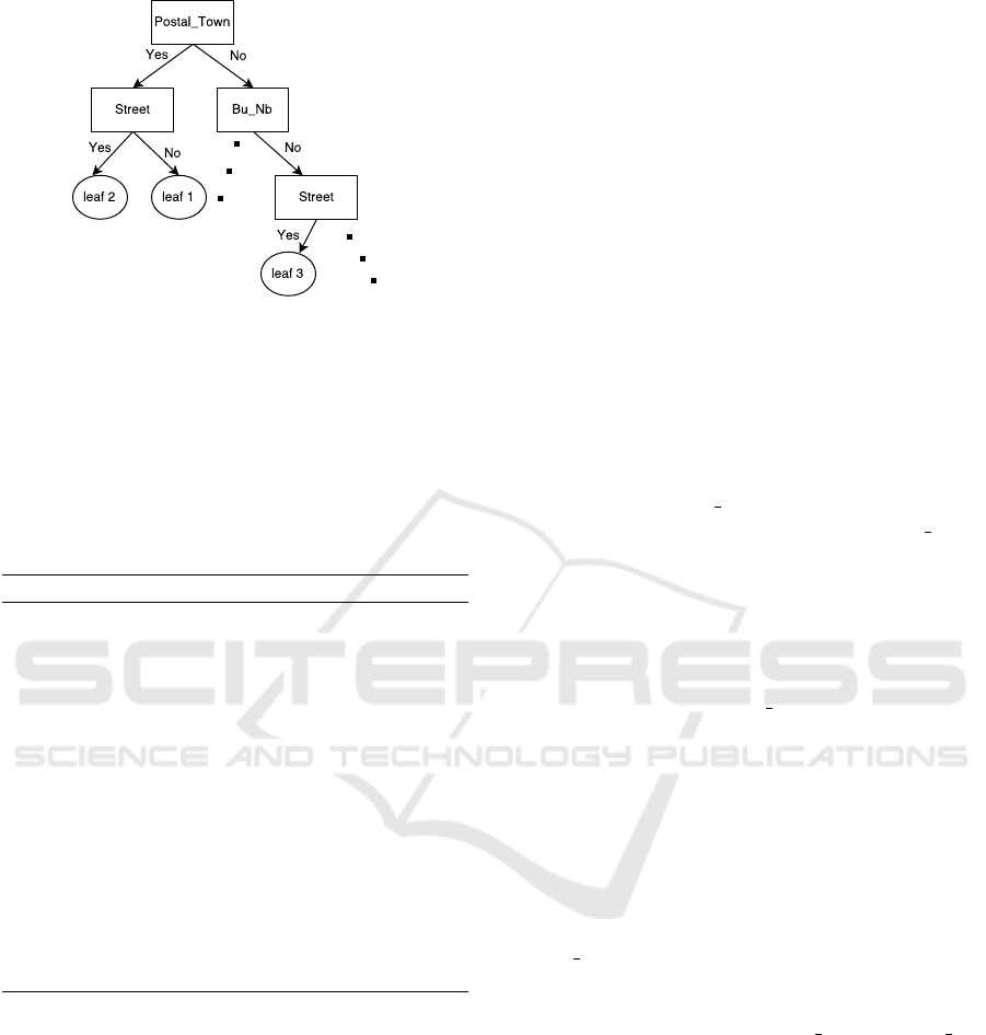
Figure 1: A toy example of search tree. Non-leaf nodes
correspond to the columns in the database. Leaf nodes are
clusters of the input queries.
columns. The second reason is that some columns
from a database might have a much wider range of
the values compared to others so that they are more
likely to get populated (possible incorrectly). Both
naive solutions are the baselines in the experiment.
Algorithm 1: Recursive Learning A Search Tree.
1: INPUT: Training Data D, Visited Columns VC
and a database R;
2: OUTPUT: SearchTreeNode nd
3: function LEARNTREE(D, VC, R)
4: if AveNumCand(D,VC, R) ≤ α then
5: Return null
6: BestC = argmax
c∈C\VC
Comp(D, c∪VC,R)
7: if Comp(D, BestColumn∪VC,R) ≥ β then
8: TreeNode nd = Node(BestColumn)
9: D
m
← containValues(D,BestC,R)
10: D
um
← D \ D
m
Unmatched Set
11: nd.left = learnTree(D
m
, BestC ∪VC,R)
12: nd.right = learnTree(D
um
, BestC ∪VC,R)
13: else Return null
14: Return nd
Since a CNF of all columns is too aggressive, we
present two algorithms that can retrieve candidates
more dynamically compared to the naive AND ap-
proach. The idea is that some attributes are more
likely to have the correct values compared to other
attributes, e.g.
homogeneous attribute values, it is better to firstly re-
trieve candidates based on reliable attributes rather
than try to generate all candidates from a single SQL
query.
A Search Tree Algorithm
Instead of constructing a CNF from all populated
columns for each query, we try to learn a hierarchical
search tree that can form a CNF with the best combi-
nations of the columns accordingly.
Definition 5.1. A Search Tree ST = (N,L,E) for a
relational entity table R is composed of a binary tree
with the non-leaf nodes N, leaf nodes L and edges E.
Each non-leaf node n ∈ N corresponds to a column c
in R. A left or right edge of the non-leaf node n de-
notes whether the node should be used to construct the
CNF or not. Given a multi-valued query ˆq, it travels
from a root node to a leaf node l ∈ L, and all the leaf
node’s ancestor nodes with left edges are considered
for the final CNF.
Now let us consider how to traverse in a search
tree. Given a tabular query, it travels to the left edge
of a node n only when the CNF of the node and all its
ancestor nodes with left edges can retrieve a positive
number of candidates from the database. For instance,
Figure 1 shows an example of a search tree. Suppose a
structured multi-valued query ˆq has at least one value
in the column Postal Town, then it will definitely
travel to the left edge of the root node Postal Town,
because there is no other ancestor nodes at this stage.
If the query ˆq does not have any value in the column
Street, it then travels to the right edge of the node
Street (leaf node 1); if the query ˆq does have some
values for the column Street, it travels to the left edge
of the node Street (leaf node 2) only when the combi-
nation of the column Postal Town and Street returns
a non-empty set of the candidates, otherwise, it also
travels to the right edge of the node Street. This is to
make sure the final CNF can always return a positive
number of the candidates even when some values are
not correctly populated.
Intuitively, each leaf node from the search tree
corresponds to a set of queries with the same choices
of the columns to form the CNF, for example,
queries that terminate at leaf 1 will only use column
Postal Town to retrieve candidates, while queries in
leaf 3 will only use column Street to retrieve can-
didates, because there is no matching values for the
other two ancestor nodes Postal Town and Bu Nb.
One thing worth noting here is that the maximum
depth of the search tree is the total number of the
columns in the database.
Now we present a recursive greedy algorithm
(shown in Alg 1) to learn a search tree from a set
of labelled queries. Each query in the training set
is labelled with a set of candidates that refer to the
same entity as the input query. The current best col-
umn is selected to maximise the completeness (line
6). There are two termination conditions of the node
expansion before it reaches the maximum depth of
the search tree, one is when the average number of
candidates (AveNumCand) is less than a pre-defined

threshold α (line 4), because there is no need to per-
form node expansion when the average number of
candidates is already quite small; the other is when
the current best column has a completeness score less
than another pre-defined threshold β (line 7) so that a
minimal completeness can be guaranteed at each step
of node expansion. If none of the early termination
conditions is satisfied, the current training data D is
then split into two separate sets depending on how the
queries follow the edges as we explained before.
Back to our running example in Section 3, given
the search tree in Figure 1, the query ˆq in Table
2 will first travel to the left edge of the root node
Postal Town because it has three possible values for
the column Postal Town. After constructing a SQL
query with both Postal Town and Street:
SELECT * FROM R WHERE
AND Street in (’Oxford Street’)
AND Postal_Town
in (’Oxford’, ’Street’, ’London’)
it returns the third record as the final result.
A MaxMatched Algorithm
We present another effective and efficient retrieval al-
gorithm, MaxMatched, that can retrieve candidates
that match to the input queries. Instead of choosing
a number of columns to form a CNF query as shown
before, the idea of the MaxMatched is to find the best
column to generate a list of candidates and then cal-
culate a similarity between each candidate tuple and
the original input query q.
The complete MaxMatched algorithm is shown in
Alg 2. An unstructured query q and the transformed
structured query ˆq are both required as input for the
MaxMatched algorithm.
We first generate an ordered list of the columns of
the database based on the completeness score from
the training data (line 4) using the same function
Comp as in line 6 of Alg 1. Out of all populated
columns, we choose the one with the best complete-
ness (highest rank) in line 5 to retrieve the first set of
the candidates from the database. The second step is
to calculate the similarity score between all retrieved
records and the unstructured query q.
The degree of similarity between the query q and a
candidate tuple is calculated by counting the number
of values from the tuple that can be found in the un-
structured query (line 9-16). Note that the maximum
number of the matching values is the total number of
the columns in the table. The whole process can be
seen as a two-stage algorithm , where the best-rank
column generate candidates at the first stage and the
tuples with maximum number of matching values are
returned at the second stage.
Algorithm 2: MaxMatched Algorithm.
1: INPUT: A free-form query q, a tabular query ˆq,
a database R and training data D;
2: OUTPUT: Candidates T
3: function MAXMATCHED(q, ˆq, R, D)
4: OC = OrderedColumns(R, D), T =
/
0
5: BestC = FirstColumnNotEmpty(OC, ˆq, R)
6: if BestC 6= null then
7: maxMatched ← 0
8: for each r ∈ R and r.BestC ∈ ˆq.BestC do
9: numMatched ← countMatched(r,q)
10: if numMatched > maxMatched then
11: Empty T
12: maxM ← numMatched
13: T = T ∪ r Add current record r
14: else if numMatched=maxM then
15: T ← T ∪ r
16: Return T
17: else Return
/
0
As for the example query “5 Oxford Street Lon-
don Englad”, we assume that the column Postal town
from Table 2 has the best completeness score so that it
is used to retrieve the first set of the candidates, which
are all five of them. Out of all tuples from Table 2,
the third record will then be returned as the final out-
put, because there are three values from the third tuple
that can be exactly found in the input query, i.e., “5”,
“Oxford Street” and “London”. The tuple a
1
has only
two values, i.e., “5” and “Oxford”, that can be found
in the query, while the tuples a
2
, a
4
and a
5
only have
one value that can be found in the query, namely “Ox-
ford”, “London” and “Street” respectively.
The MaxMatched algorithm is more flexible than
choosing a fixed number of columns as in the
SearchTree algorithm, however, it relies on the best
ranked column to retrieve the first set of the candi-
dates.
6 EXPERIMENTS
We tested effectiveness and efficiency of our sys-
tem on an official UK address database called Post-
code Address File (PAF, 2017) provided by the UK
Royal Mail. The PAF database maintains over 29
million residential and commercial addresses, where
there are 12 columns in the main table. Column
co name is used to store company names, and the rest
of the columns are responsible for addresses. Three
columns pc
dist (first part of post code), pc sffx (sec-
ond part of post code) and dp sffx (deliver point) form
an unique ID for each address. Columns, such as
road name Rd Nm and sub-road name Sb Rd, share

Table 3: Number of tokens and free tokens per query.
Datasets # of Tokens # of Free Tokens
YellowPage 13.82 4.35
Company 12.13 3.68
a large vocabulary, more specifically, most of the val-
ues from the column Sb Rd can be found in the col-
umn Rd Nm. Another thing worth noting is that col-
umn building name Bu Nm has a much wider range
of values compared to the other address columns, i.e.,
the number of distinct values of the column Bu Nm
is 1,048,576 while the second largest column Rd Nm
has only 320,017 distinct values.
Two real-world datasets, each of which contains
a list of UK company records, are used as the input
entity queries. One contains 100 furniture company
records extracted from the UK Yellow Pages web-
site (YellowPage, 2017) and the other is a Company
dataset which contains 200 UK company records
from a private company database. The datasets are
split equally into training and test sets. The goal is to
search for the tuples in the PAF database that refer to
the same entity as the input query.
As shown in Table 3, the average numbers of to-
kens per query for our entity search/match evaluation
are significantly larger compared to the ones in key-
word search literature (usually less than 6). Also web
and commercial data is often not standardised and
will differ in structure when compared to reference
sources such the PAF dataset. Table 3 shows nearly
a quarter of the tokens for each query could not be
mapped to any of the columns in the database.
As said in Section 5, the effectiveness of the algo-
rithm is measured by completeness, which determines
whether the returned set of the tuples T cover all cor-
rect tuples T
∗
, which is manually decided by our do-
main expert. For each query, the completeness is 1 if
T
∗
⊂ T . We then computed the fraction of queries that
have full completeness. The efficiency is measured by
the average number of returned tuples.
There are three main baseline approaches used
here. As explained in Section 4, the structured an-
notation method first converts a text query into many
structured queries, where each structured query has
non-overlapping values that cover the entire input
query. Each structured query is then connected with
OR semantic. On the other hand, NaiveAnd and
NaiveOr methods, which are described in Section 5,
rely on a single structured query with potentially over-
lapping values between columns.
The comparison results of different methods are
shown in Tables 4 and 5. For the SearchTree algo-
rithm, the two hyper-parameters α and β are set to
Table 4: Comparison results for the Yellow Pages dataset.
Completeness #Cand
NaiveAnd 0 0
NaiveOr 1.0 491694
Structured Annotation 0.24 1.07
SearchTree 0.92 9
MaxMatched 1.0 7
Table 5: Comparison results for the company dataset.
Completeness #Cand
NaiveAnd 0 0
NaiveOr 0.91 54953
Structured Annotation 0.29 1.6
SearchTree 0.83 285
MaxMatched 0.87 287
be 30 and 0.85 respectively, which shows good per-
formance for both datasets. The NaiveAnd method
returns an empty set for both datasets, which shows
that it is too restrictive to consider all columns from
the structured queries. The NaiveOr method, on the
other hand, achieved the best completeness for both
datasets, but also returned a large number of can-
didates. As shown in Table 4, the average num-
ber of candidates of the NaiveOr method is hun-
dreds of thousands for the Yellow Pages dataset, but
the SearchTree and MaxMatched methods only re-
turn less than 10 candidates per query. The com-
pleteness rates of the structured annotation method
are only 24% and 29% for the two datasets, which
are significantly smaller compared to the SearchTree
and MaxMatched algorithms. This is due to the fact
that some tokens from the query are wrongly mapped
to the columns, resulting in none of the structured an-
notations of the query being a possible interpretation
of the query.
There are more candidates generated per query
for the Yellow Pages dataset compared to the com-
pany dataset when applying the NaiveOr method, be-
cause the data from the Yellow Pages has much less
noise than the company dataset, which means more
matching values appear in the structured queries. In
summary, both SearchTree and MaxMatched meth-
ods dramatically reduce the number of candidates as
compared to NaiveOr approach while still maintain-
ing a competitive completeness.
As the columns pc dist and pc sffx are part of the
unique identifier for an address entity, we also tested
our methods without considering these two ID-like
columns. Table 6 shows that a much larger number of
candidates were returned and completeness was re-

Table 6: Results without columns pc dist and pc sffx.
Completeness #Cand
YellowPage
SearchTree (NoPC) 0.81 2763
MaxMatched (NoPC) 0.87 2876
Company
SearchTree (NoPC) 0.67 4512
MaxMatched (NoPC) 0.73 1962
Table 7: Average Execution time.
Yellow Page (s) Company (s)
NaiveAnd 0.11 0.28
NaiveeOr 239.36 300.57
SA 13.7 1.05
SearchTree 2.51 4.67
MaxMatched 0.82 0.68
duced compared to the case where all columns are
considered.
Finally, the average execution times per query for
the different algorithms are shown in Table 7. As
expected, NaiveOr has the largest retrieval time be-
cause of the large number of possible candidates. The
SearchTree method generally takes more time to re-
trieve candidates than the MaxMatched, because it
has to decide which branch to follow at each non-
leaf node by checking whether the current combina-
tion of the ancestor nodes can generate a non-empty
set, while the MaxMatched method only has to enu-
merate all candidates constrained by the best column.
7 CONCLUSIONS
We have presented an effective and efficient approach
to address the problem of entity search/match over
RDBs. We showed that structured annotation of the
query is not suitable when there is redundant infor-
mation in the input queries that could mislead the
interpretations. Two supervised retrieval methods
were proposed to retrieve candidate tuples based on a
multi-valued structured query. The results of the com-
prehensive evaluation for the large-scale database and
two real-world datasets showed that our methods can
achieve a good trade-off between generating correctly
matching candidate and the retrieval time.
REFERENCES
Agrawal, S., Chaudhuri, S., and Das, G. (2002). DBX-
plorer: A System for Keyword-Based Search over Re-
lational Databases. In Proceedings of the 18th Inter-
national Conference on Data Engineering.
Balog, K., de Vries, A. P., Serdyukov, P., and Wen, J.-R.
(2012). The first international workshop on entity-
oriented search (eos). In ACM SIGIR Forum, vol-
ume 45, pages 43–50. ACM.
Blanco, R., Mika, P., and Vigna, S. (2011). Effective and
Efficient Entity Search in RDF data. In Proceedings
of International Semantic Web Conference.
Ferragina, P. and Scaiella, U. (2010). TAGME: On-the-fly
Annotation of Short Text Fragments (by Wikipedia
Entities). In Proceedings of the 19th ACM interna-
tional conference on Information and knowledge man-
agement. ACM.
Golenberg, K., Kimelfeld, B., and Sagiv, Y. (2008). Key-
word Proximity Search in Complex Data Graphs. In
Proceedings of the SIGMOD international conference
on Management of Data. ACM.
Hristidis, V., Gravano, L., and Papakonstantinou, Y. (2003).
Efficient IR-style keyword search over relational
databases. In Proceedings of the 29th International
Conference on Very Large Data Bases.
Hristidis, V. and Papakonstantinou, Y. (2002). Discover:
Keyword search in relational databases. In Proceed-
ings of the 28th International Conference on Very
Large Data Bases, VLDB ’02. VLDB Endowment.
Kim, J., Xue, X., and Croft, W. B. (2009). A Probabilistic
Retrieval Model for Semistructured Data. In Euro-
pean Conference on Information Retrieval. Springer.
Liu, F., Yu, C., Meng, W., and Chowdhury, A. (2006). Ef-
fective Keyword Search in Relational Databases. In
Proceedings of the International Conference on Man-
agement of Data. ACM.
PAF (2017). Royal mail postcode address file.
https://www.poweredbypaf.com/.
Pound, J., Mika, P., and Zaragoza, H. (2010). Ad-hoc Ob-
ject Retrieval in the Web of Data. In Proceedings of
the 19th international conference on World Wide Web.
Sarkas, N., Paparizos, S., and Tsaparas, P. (2010). Struc-
tured Annotations of Web Queries. In Proceedings of
the International Conference on Management of data.
ACM.
Simitsis, A., Koutrika, G., and Ioannidis, Y. (2008). Pr
´
ecis:
From unstructured keywords as queries to structured
databases as answers. The VLDB Journal, 17(1).
Talburt, J. R. (2011). Entity Resolution and Information
Quality. Elsevier.
YellowPage (2017). UK yellow page website.
https://www.yell.com/.
Yu, J. X., Qin, L., and Chang, L. (2010). Keyword Search
in Relational Databases: A Survey. IEEE Data Engi-
neering Bulletin, 33(1).
