Towards a Better Understanding of Deep Neural Networks
Representations using Deep Generative Networks
J
´
er
´
emie Despraz
1,2
, St
´
ephane Gomez
1,2
, H
´
ector F. Satiz
´
abal
1
and Carlos Andr
´
es Pe
˜
na-Reyes
1,2
1
School of Business and Engineering Vaud (HEIG-VD), University of Applied Sciences of Western Switzerland (HES-SO),
Yverdon-les-Bains, Switzerland
2
Computational Intelligence for Computational Biology (CI4CB), SIB Swiss Institute of Bioinformatics,
Lausanne, Switzerland
Keywords:
Deep-Learning, Convolutional Neural Networks, Generative Neural Networks, Activation Maximization,
Interpretability.
Abstract:
This paper presents a novel approach to deep-dream-like image generation for convolutional neural networks
(CNNs). Images are produced by a deep generative network from a smaller dimensional feature vector. This
method allows for the generation of more realistic looking images than traditional activation-maximization
methods and gives insight into the CNN’s internal representations. Training is achieved by standard backprop-
agation algorithms.
1 INTRODUCTION
Artificial deep-neural networks have proven ex-
tremely successful in a wide variety of tasks but re-
main extremely opaque in terms of what they learn
and how they use their acquired knowledge to make
predictions. In particular, without any insight into
the network, the task of determining whether it has
properly integrated a specific concept is very difficult
and the subsequent validation of the method for crit-
ical activities is not possible. Furthermore, without
a tool to interrogate the network concerning what it
has learned from a given dataset, it is very difficult
to transfer the acquired knowledge from the network
parameters to a human user. These considerations
demonstrate the need for methods that would allow
us to gain better insight into deep-neural networks.
This paper makes a step in that direction with the
introduction of a method that can produce preferred
inputs to a trained network, thus enabling the creation
of representative and interpretable data that reflects
the network’s internal representations.
2 RELATED WORK
Extensive work has been recently done towards better
understanding artificial neural networks, especially in
the domain of convolutional neural networks (CNN).
In particular, several methods have been proposed
in order to gain insight into the internal representa-
tions and decision-making processes of the neural net-
works. Yosinski et al. (Yosinski et al., 2015) devel-
oped a tool to visualize filter activation given an in-
put image. They also introduced a method for gradi-
ent ascent that modifies each single pixel of the input
as to maximize a given neuron activation, resulting
in human interpretable but fairly unrealistic-looking
images of preferred inputs (see Figure 1). Other re-
searchers have developed methods to highlight spe-
cific regions of interest of an input image. Sprin-
genberg et al. (Springenberg et al., 2014) introduced
guided-backpropagation, a modified implementation
of the standard backpropagation method, that empha-
sizes parts of the image connected to a given class
by a sequence of strictly positive weights. Zeiler et
al. (Zeiler and Fergus, 2014) also introduced a novel
visualization technique based on deconvolution and
filter activation. Simonyan et al. (Simonyan et al.,
2013) used gradient backpropagation on the original
network input to compute saliency maps and to ex-
tract relevant features from images.
A more recent approach that has been very suc-
cessful at creating patterns closely matching the prop-
erties of real images are generative methods. This
field is very dynamic and methods have evolved
quickly, from the generation of images by evolution-
Despraz J., Gomez S., Satizà ˛abal H. and PeÃ
´
sa-Reyes C.
Towards a Better Understanding of Deep Neural Networks Representations using Deep Generative Networks.
DOI: 10.5220/0006495102150222
In Proceedings of the 9th International Joint Conference on Computational Intelligence (IJCCI 2017), pages 215-222
ISBN: 978-989-758-274-5
Copyright
c
 2017 by SCITEPRESS – Science and Technology Publications, Lda. All rights reserved

ary algorithms using direct and indirect encodings
(Nguyen et al., 2015), to more complex reconstruc-
tion techniques (Mahendran and Vedaldi, 2015), to
the current state-of-the-art generative adversarial net-
works (GANs) (Radford et al., 2015).
Studies on GANs have demonstrated that deep-
generative networks can be used to create images
exhibiting properties very similar to natural ones,
sometimes making them indistinguishable to humans
(Denton et al., 2015). In this context, other re-
searchers have developed methods capable of gen-
erating preferred inputs for activation maximization.
In particular, a method similar to the one presented
herein has been recently proposed by Nguyen et al.
(Nguyen et al., 2016) that allows generating photo-
realistic images from a deep-generative neural net-
work. In order to obtain well-structured images, they
used part of a GAN network, previously trained, to
generate sets of images similar to the ones they tar-
geted. To ensure the convergence of the optimization
to a realistic-looking image, they further constrained
the inputs to be within a well defined range, allowing
only for values that trigger neuron responses close to
the ones measured with images from the train dataset.
It is only upon our own work’s completion that we
became aware of such a closely-related work, carried
out in parallel to ours. While we have chosen similar
approaches, some points differ. In particular, our im-
plementation used less restrictive constraints on the
parameters and considered configurations where the
network’s weights were randomly initialized and op-
timized. Also, we implemented our method on top of
the very deep VGG-16 model (Simonyan and Zisser-
man, 2014), a model that was not considered in the
aforementioned study.
Details on our specific implementation are pre-
sented in Section 3.
3 METHODS
The core idea of the proposed method is to couple
a generative deep-neural network (G) to a pretrained
CNN (D) as depicted schematically on Figure 2. The
weights of the classifier D are assumed to be already
optimized for a specific classification task and remain
fixed. The activation functions are also kept, except
for the last classification layer where the usual soft-
max functions are replaced with rectified linear units
(ReLUs).
The resulting coupled network has one input
layer: a 1-dimensional feature vector, and two out-
put layers: an image whose dimensions are identical
to D’s inputs and a series of activations for each out-
(c)
(a)
(b)
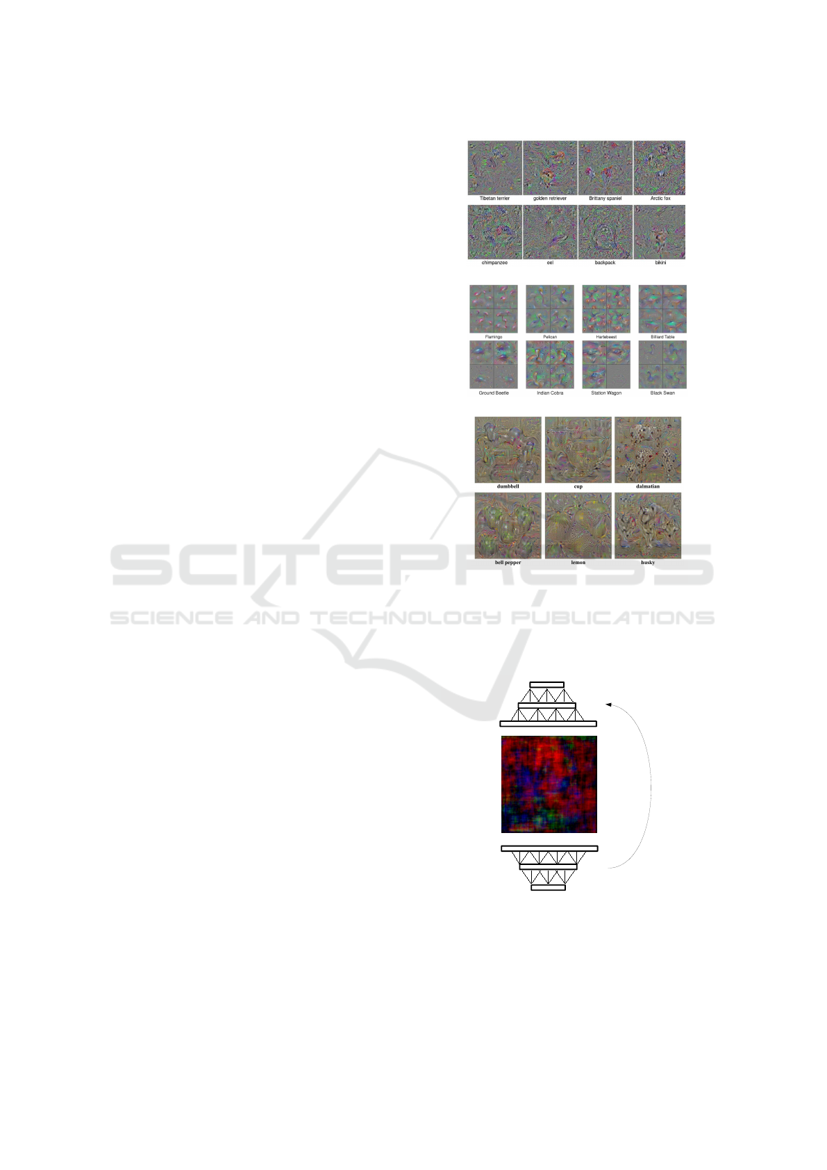
Figure 1: Examples from previous works showing preferred
input images constructed by activation maximization meth-
ods that do not rely on a deep generative network. (Images
(a), (b), and (c) from (Nguyen et al., 2015; Yosinski et al.,
2015; Simonyan et al., 2013), respectively).
Generator
Network (G)
Trained
Classifier (D)
Targeted
optimization
through
backpropagation
Figure 2: Architecture of a coupled generative-
discriminative network. The generative network G
creates images from an input feature vector and these
images are fed to the already-trained discriminator D. The
weights of D are fixed and the entire coupled network
is trained with a specific loss function so as to make G
generate images that yield the desire response from D.

put neuron of D. The task of G is to generate an image
that maximizes the activation of a particular output
neuron of D:
feature space −→
G
image −→
D
class-neuron activation
The transformation from feature space to image space
is a mapping from R
m
to R
n×n
, and is achieved
through a series of upsampling, convolution, and
batch normalization operations. The feature vector f
is built as:
( f
1
,..., f
m
)
T
=

α
1
ε( f
(0)
1
),...,α
m
ε( f
(0)
m
)

T
(1)
where the expression ε(·) is a function introducing
a random Gaussian perturbation (similar to jitter in
other works (Mahendran and Vedaldi, 2016)), f
(0)
i
∈
R are constant parameters, and α
i
∈ R are parameters
to be optimized.
In order to generate an image that maximizes the ex-
pression of a single target class c
i
, we define the loss
function of our coupled network as:
loss = −a(c
i
) + λ
∑
i6= j
a(c
j
) + R(ξ) (2)
where a(·) is the target neuron activation function,
λ ∈ R
+
is a factor penalizing the activation of other
classes, and R(ξ) is a regularizer defined on a subset
of parameters ξ of the generator network.
The loss function is then minimized using stan-
dard backpropagation methods over the entire cou-
pled network. The choice of ReLU as the activation
function on the last layer is justified because it pre-
vents a decrease in the loss function due to negative
contributions of non-targeted neurons c
j
. Therefore,
in the case where a(c
j
) = 0 ∀ j 6= i (i.e. all classes
other than i do not contribute to the loss), the opti-
mization should favor a maximal expression of the
target neuron c
i
. Convergence can be controlled by
ensuring that a(c
i
) > 0 ∀t thus removing the risk of
having d(loss) = 0 at some point in the optimization
which would prevent full convergence to the optimum
solution.
We considered two distinct approaches for the con-
struction of network G. One where we initialize each
layer with random weights and biases, and one where
we extract G from a trained denoising autoencoder
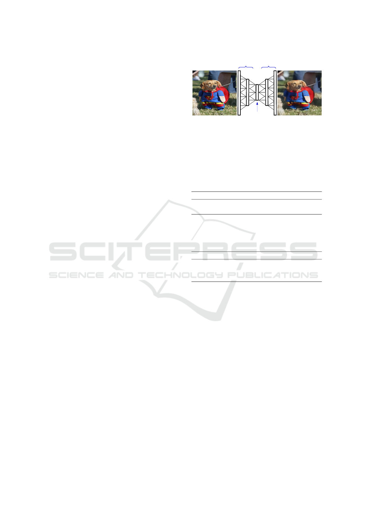
(Vincent et al., 2010) as illustrated in Figure 3. The
advantage of the second method is that the network
G has already learned a mapping from the input fea-
ture vector space to a set of natural images. There-
fore, the optimization problem is reduced to the task
of finding coordinates of the feature vector that yield
the strongest activation of the target neuron.
Table 1 lists the parameters and optimizers used
for training. The detailed network architecture can be
found in the Appendix.
Encoder (E) Generator (G)
Feature
vector
Figure 3: Architecture of the denoising autoencoder (Vin-
cent et al., 2010). It is composed of an encoder network (E)
that generates a feature vector representation from the noisy
input image and a generative network (G) that attempts to
regenerate the original image from the feature vector.
Table 1: Implementation details and parameters used for
optimization of the coupled deep-networks in the untrained
and pretrained configurations.
NO PRETRAINING WITH PRETRAINING
Variables 5.240.841 3.200
Optimizer AdaMax Stochastic gradient
(Kingma and Ba, 2014) descent
Parameters learning rate = 0.002, learning rate = 0.01,
β
1
= 0.9, momentum = 0.1,
β
2
= 0.999, Nesterov momentum,
decay = 0, decay = 0
ε = 10
−08
Initial conditions f = 1 f = 0
Noise parameters type = additive, type = multiplicative,
µ = 0, µ = 1,
σ = 2 σ = 0.05
It is worth noting that this method is not limited to
class description as it can be applied identically to any
neuron or group of neuron activations in the CNN by
simply adapting the loss function in Equation 2. As a
result, it allows the generation of images representing
arbitrary-level (low, mid, or high) features learned by
a CNN as well as any combination of them.
4 RESULTS
In order to test our method, we used the freely avail-
able, very deep VGG-16 model (Simonyan and Zis-
serman, 2014) as a target discriminator and we con-
structed a generator whose full architecture is de-
scribed by Table 2 in the Appendix. To implement,
test, and optimize the deep-neural networks, we used
the open-source library Keras (Chollet, 2015) with the
Tensorflow (Abadi et al., 2016) backend. Sections 4.1
and 4.2 present the results obtained by optimizing the
loss function for network G as defined by Equation 2,
without and with pretraining, respectively.

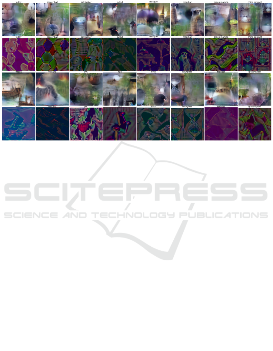
Figure 4: Selection of images generated by both methods (lines 1 and 3 are outputs of the pretrained network). Each row
contains two couples of images sharing the same target class label. Images created with the pretrained network are less
saturated, and often possess a more complex spatial structure making them visually more resemblant to natural images. This
image is best viewed in color/screen.
4.1 Without Pretraining
In this setup, the regularizer expression of Equation 2
becomes:
R(ξ) = 0.01`
1
(γ) = 0.01
3
∑
k=1
|γ
k
| (3)
where γ
k
are the weights associated with the 3 chan-
nels of the generated image. This expression prevents
the possible drift toward over-saturated images. A
few examples of generated images are presented in
Figure 4.
Images generated with this method can be, for the
most part, easily interpreted by a human, as the main
features of the class generally appear quite clearly. It
is also worth noting that the network is capable of cre-
ating a wide variety of shapes and textures that are
close to those seen on natural images, despite the fact
that it has never “seen” an actual image and therefore
has no preexisting internal representations of these
features.
However, these images also often display unrealis-
tic colors as well as low spatial ordering. Most of the
time, we observed typical class patterns that are re-
peated over the entire image. This is probably partly
due to the fairly large amount of noise that is gener-
ated on the feature vector that has been deemed nec-
essary to ensure convergence to a visually interesting
solution. These issues are, in part, tackled by intro-
ducing pretraining.
4.2 With Pretraining
We used a dataset of dog pictures from ImageNet
(Russakovsky et al., 2015) to train the denoising au-
toencoder illustrated in Figure 3. The advantage of
the dog dataset with respect to some other classes of
ImageNet is the variety of pictures it contains. It com-
prises for instance many subclasses corresponding to
several different dog breeds, each with its special at-
tributes (color, shape, fur type, size, etc.) taken in
various contexts and locations. This allowed the au-
toencoder to be exposed to a wide variety of images,
thus reinforcing its ability to reconstruct the different
features present in the VGG-16 classes.
Before feeding the images to the network, Gaus-
sian noise was added to improve the quality of the
learning process (Vincent et al., 2010) and error was
measured as the mean-squared Euclidian distance be-
tween the input and the reconstructed image. This
approach is relatively light and easy to implement.
However, it has the disadvantage of leading the gener-
ator G to produce blurry images, cutting off some high
frequency components of the original input. In this
configuration, the regularizer expression from Equa-
tion 2 becomes:
R(ξ) = 0.1`
2
(α) = 0.1
s
N
∑
k=1
α
2
k
(4)
where α
k
are the weights of the first layer (see Equa-
tion 1) and N is the length of the input feature vector.

This expression keeps the coordinates of the feature
vector in a reasonable range. Furthermore, we assume
that the network has learned a good-enough mapping
from the feature space to the real-image space. Thus,
with the exception of the first layer, we fix the weights
of the entire autoencoder, hence dramatically reduc-
ing the amount of parameters to be trained. A few
examples of generated images are presented in Fig-
ure 4.
Interestingly, images produced with this setup
have much more realistic colors and seem to have a
greater level of structure with respect to the imple-
mentation shown in Section 4.1. For many of the gen-
erated pictures, a posteriori class identification can be
done without too much effort. Also, the network is
able to reproduce patterns that have not been previ-
ously “seen” (and therefore, that could not have been
learned a priori) as it was trained exclusively with pic-
tures belonging to the dog class.
However, it also appears that the network is not
able to reproduce sharp details and has trouble repro-
ducing high frequency components observed in natu-
ral images. This limitation is most probably linked
to the pretraining phase of the autoencoder where
the choice of RMSE as loss function did not account
enough for high frequency terms.
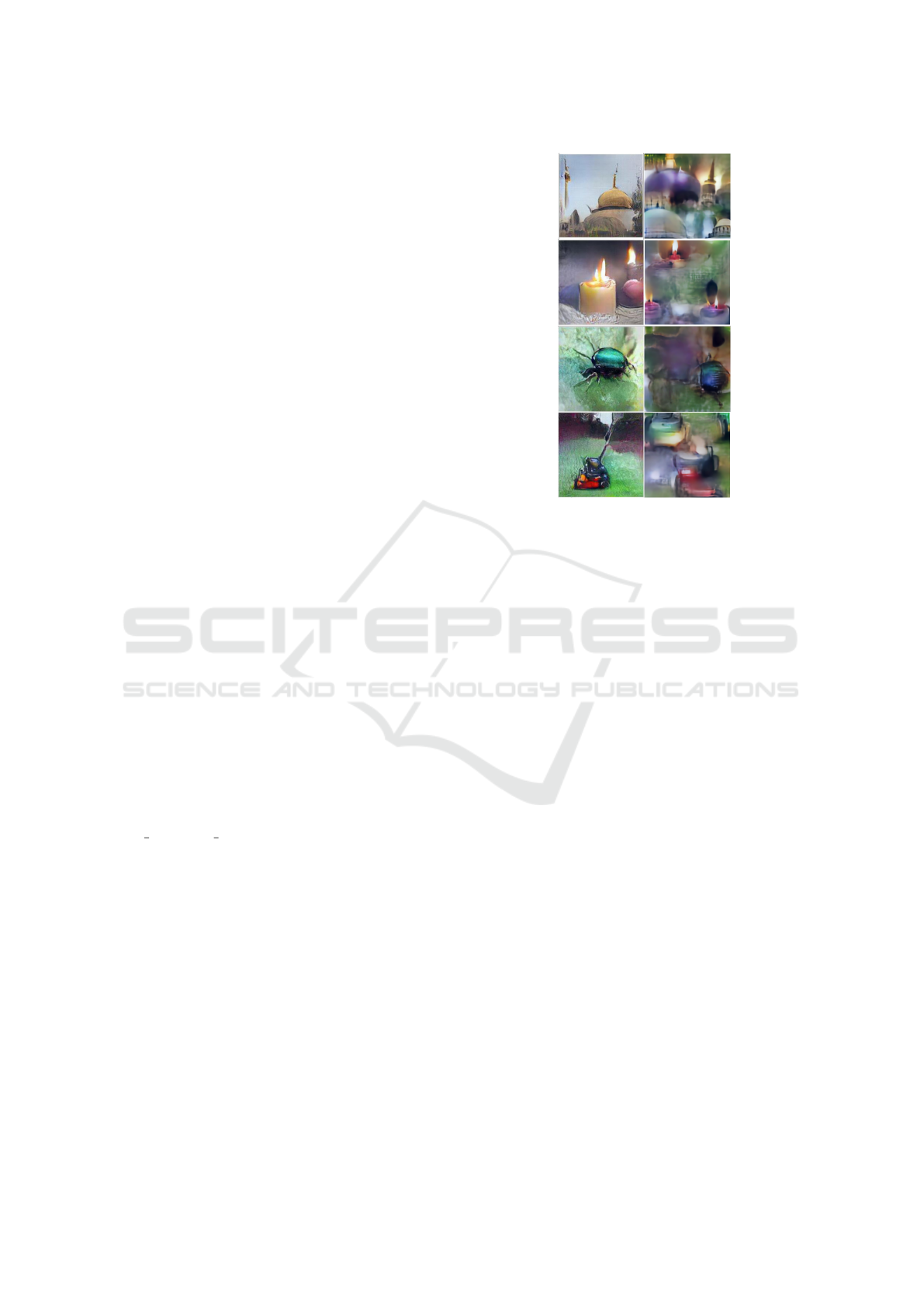
A comparison of our method with (Nguyen et al.,
2016) (see Figure 5), suggests that our results might
be improved further, for instance by using a gener-
ative network previously trained to reproduce highly
realistic images. While the level of details provided
by our method is not as high as in Nguyen’s, we ob-
serve similar features on the generated images of a
given class.
The original code as well as images for all the
1,000 classes of the VGG-16 network were gener-
ated with both of the presented methods and are
available for download at https://github.com/jdespraz/
deep generative networks.
5 DISCUSSION AND
APPLICATIONS
As we have seen, the method introduced in this paper
allows the generation of images that have a structure
similar to natural images. This represents a great ad-
vantage with respect to most generative techniques,
such as deep-dreams and other input-based optimiza-
tions methods (see Figures 1 and Figure 4 for com-
parison). Also, since it does not require any modifi-
cations or re-optimization of the discriminative net-
work (as in GANs for example), the method does not
alter the original network and can be applied effec-
Figure 5: Comparison with (Nguyen et al., 2016) (left
column) and our method (right column) for the classes
Mosque, Candle, Leaf Beatle, and Lawn Mower.
tively directly by coupling a generative network and
using standard backpropagation algorithms. The im-
plementation is therefore relatively simple and not ex-
cessively costly in terms of computation time.
In addition, our method enables various new
techniques of deep-neural network analysis that we
present in this section.
5.1 Interpretability
The analysis of the generated images allows for some
degree of interpretation of the discriminator network’s
internal representation of the classes. In particular, it
appears that some classes have been trained with bi-
ased samples, and this bias is reflected in the gener-
ated images. Typical examples are presented in Fig-
ures 6 and 7. Interestingly, it seems that the bias is
more strongly expressed with the pretrained network.
We observe for example that the classes crib and
cradle both lead the network to generate images of a
baby, the miniskirt class seems to react to naked legs,
and muzzle includes information about dogs’ faces.
Similarly, for musical instruments, as illustrated in
Figure 7 by the harmonica class, they appear most of
the time in the training set held by musicians and, as
a result, the network seems to include in these classes
the arms and fingers as if they were part of the object.
The same can be observed with the class tench where
images in the train dataset contain many instances of
fishermen holding the fish in their hands and gener-
ated images do therefore include properties of the fish

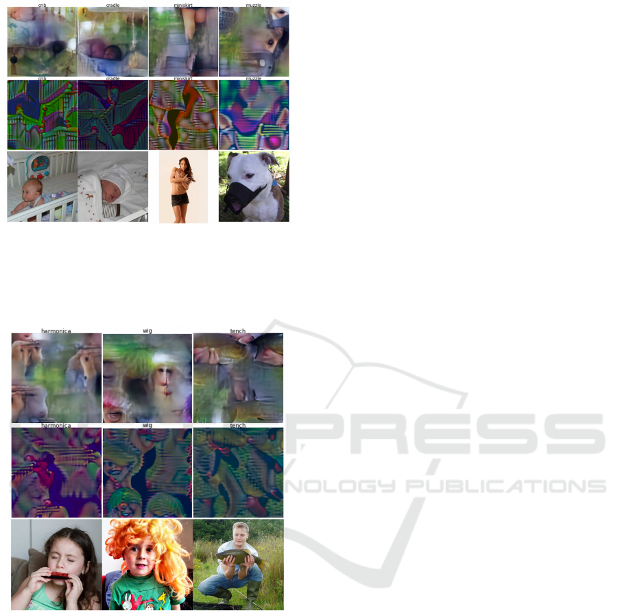
Figure 6: First selection of images displaying some bias
in the network’s internal representations. Row 1 shows the
outcome of the pretrained network, row 2 the untrained net-
work, and row 3 a typical example of the training dataset.
Biases seem to appear more clearly in the outputs of the
trained network.
Figure 7: Second selection of images displaying some bias
in the network’s internal representations. Row 1 shows the
outcome of the pretrained network, row 2 the untrained
network and row 3 a typical example of the train dataset.
Biases seem to appear more clearly in the outputs of the
trained network.
as well as human fingers.
Being able to interpret the network’s acquired knowl-
edge in such a way is extremely useful as it allows us
to improve the quality of the training by detecting and
removing observed biases, leading eventually to more
robust, accurate, and reliable predictions.
5.2 Knowledge Discovery
This method can potentially be used to gather new
(possibly unknown) information about the training
data. For example, let us assume the scenario where a
deep-neural network has been trained to detect and
classify patients with lung cancer based on radio-
graphic images, classifying them into two classes,
“ill” or “healthy”. If we were to generate images
that strongly activate the “ill” class of this network,
we could have an idea of the signs the network has
learned to recognize cancerous cells, potentially dis-
covering new features of cancer images.
5.3 Feature Explanation
In the domain of rule or feature extraction, one tries
to extract knowledge from deep-neural networks in
order to better explain their behavior. With CNNs,
the extracted information is sometimes represented in
the form of rules consisting of a set of weighted fil-
ter indices. While these rules may accurately reflect
the network’s behavior, they are often difficult to un-
derstand; filters are often not easily interpretable and
their linear combinations can be even more obscure.
In this context, our method could allow the genera-
tion of images displaying a graphical representation
of a set of extracted filters, thus allowing for a more
easily interpretable explanation rather than having a
simple set of feature identifiers. This could easily be
achieved simply by replacing the activation of neuron
c
i
in Equation 2 by a group of neurons corresponding
to a set of features.
Figure 8 illustrates some of the representations ob-
tained for a set of filters on two different network
layers. It clearly highlights the hierarchical struc-
ture of the network since filters close to the input re-
act strongly to simple patterns whereas filters closer
to the output display much more complex structures.
Some of these high-level features are also easily rec-
ognizable as for instance ears, eyes, hands or clothes.
5.4 Generative Tools
Another usage of this method can be the generation
of compound images, containing features of several
classes. Some examples of such images are presented
in Figure 9 where we constructed images that max-
imize the output of two distinct classes. Generated
images display attributes of the two classes, and these
characteristics are sometimes present in the texture
(such as the jigsaw puzzle) or mixed in a single ob-
ject (such as with the ostrich and the bullfrog).

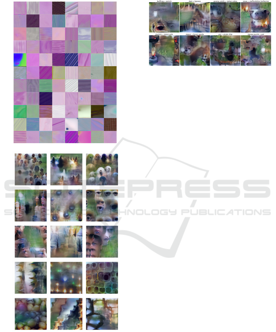
(a) Generated images for filters of the 9th layer
(b) Generated images for filters of the 26th layer
Figure 8: Selection of generated images that maximize filter
responses of a given network layer. As expected, preferred
images for layers close to the input exhibit simple patterns
(straight lines, uniform colors) and the complexity of these
patterns increases as we get deeper into the network. Some
of the high-level features such as eyes, hands, ears or dog’s
faces can easily be recognized.
Figure 9: Some examples of images generated to maximize
the activation of two classes. Resulting images display at-
tributes of both classes.
We can imagine a wide variety of applications for a
tool capable of mixing various image attributes, from
a pure artistic perspective of creating new content to a
more pragmatic approach of generating preferred in-
puts for specific CNN layers or filters. In particular, it
would be very interesting to couple this approach with
a feature selection tool that would generate images
corresponding to a particularly relevant feature or a
combination of those. Besides, several methods of
feature extraction have already been successfully de-
veloped and implemented (Ribeiro et al., 2016; Zhou
et al., 2015).
6 CONCLUSION
We have presented a method that allows the genera-
tion of images that trigger a strong response of a tar-
get neuron in a trained classifier. We have considered
an approach where the generative network is trained
from scratch, and another where it was first trained
to generate natural images from a lower dimensional
feature vector.
The resulting images display some degree of
structure and detail that is similar to real images and
allows interpretations of the network’s internal repre-
sentations. We have demonstrated that complex lev-
els of structure and patterns can be generated without
ever being “seen” by a deep-neural network, simply
by minimizing a well chosen loss function.
Finally, we presented potential applications of this
method in neural network interpretation, data analysis
and image generation. In particular, we have demon-
strated through examples the usefulness of such an ap-
proach to detect biases in the network’s internal rep-
resentations.

ACKNOWLEDGEMENTS
This work was supported by the Hasler Fundation,
project number 16015.
REFERENCES
Abadi, M., Agarwal, A., Barham, P., Brevdo, E., Chen, Z.,
Citro, C., Corrado, G. S., Davis, A., Dean, J., Devin,
M., et al. (2016). Tensorflow: Large-scale machine
learning on heterogeneous distributed systems. arXiv
preprint arXiv:1603.04467.
Chollet, F. (2015). Keras.
Denton, E. L., Chintala, S., Fergus, R., et al. (2015). Deep
generative image models using a laplacian pyramid of
adversarial networks. In Advances in neural informa-
tion processing systems, pages 1486–1494.
Kingma, D. and Ba, J. (2014). Adam: A method
for stochastic optimization. arXiv preprint
arXiv:1412.6980.
Mahendran, A. and Vedaldi, A. (2015). Understanding
deep image representations by inverting them. In
2015 IEEE conference on computer vision and pattern
recognition (CVPR), pages 5188–5196. IEEE.
Mahendran, A. and Vedaldi, A. (2016). Visualizing
deep convolutional neural networks using natural pre-
images. International Journal of Computer Vision,
120(3):233–255.
Nguyen, A., Dosovitskiy, A., Yosinski, J., Brox, T., and
Clune, J. (2016). Synthesizing the preferred inputs
for neurons in neural networks via deep generator net-
works. In Advances in Neural Information Processing
Systems, pages 3387–3395.
Nguyen, A., Yosinski, J., and Clune, J. (2015). Deep neural
networks are easily fooled: High confidence predic-
tions for unrecognizable images. In 2015 IEEE Con-
ference on Computer Vision and Pattern Recognition
(CVPR), pages 427–436. IEEE.
Radford, A., Metz, L., and Chintala, S. (2015). Unsu-
pervised representation learning with deep convolu-
tional generative adversarial networks. arXiv preprint
arXiv:1511.06434.
Ribeiro, M. T., Singh, S., and Guestrin, C. (2016). ” why
should i trust you?”: Explaining the predictions of any
classifier. arXiv preprint arXiv:1602.04938.
Russakovsky, O., Deng, J., Su, H., Krause, J., Satheesh, S.,
Ma, S., Huang, Z., Karpathy, A., Khosla, A., Bern-
stein, M., et al. (2015). Imagenet large scale visual
recognition challenge. International Journal of Com-
puter Vision, 115(3):211–252.
Simonyan, K., Vedaldi, A., and Zisserman, A. (2013).
Deep inside convolutional networks: Visualising im-
age classification models and saliency maps. arXiv
preprint arXiv:1312.6034.
Simonyan, K. and Zisserman, A. (2014). Very deep con-
volutional networks for large-scale image recognition.
arXiv preprint arXiv:1409.1556.
Springenberg, J. T., Dosovitskiy, A., Brox, T., and Ried-
miller, M. (2014). Striving for simplicity: The all con-
volutional net. arXiv preprint arXiv:1412.6806.
Vincent, P., Larochelle, H., Lajoie, I., Bengio, Y., and
Manzagol, P.-A. (2010). Stacked denoising autoen-
coders: Learning useful representations in a deep net-
work with a local denoising criterion. Journal of Ma-
chine Learning Research, 11(Dec):3371–3408.
Yosinski, J., Clune, J., Nguyen, A., Fuchs, T., and Lipson,
H. (2015). Understanding neural networks through
deep visualization. arXiv preprint arXiv:1506.06579.
Zeiler, M. D. and Fergus, R. (2014). Visualizing and under-
standing convolutional networks. In European Con-
ference on Computer Vision, pages 818–833. Springer.
Zhou, B., Khosla, A., Lapedriza, A., Oliva, A., and Tor-
ralba, A. (2015). Learning deep features for discrimi-
native localization. arXiv preprint arXiv:1512.04150.
APPENDIX
The network detailed architecture is presented in
this section. You can also access the original source
code as well as the entire set of generated images at
https://github.com/jdespraz/deep generative networks
Table 2: Detailed generative network architecture (G).
LAYER DIM
Input Vector 1 × 3200
Gaussian Noise
Locally Connected 1D 1 × 1
Reshape 128 × 5 × 5
Upsampling 2×2
Convolution 2D 512 × 2 × 2
Batch Normalization
Convolution 2D 512 × 2 × 2
Batch Normalization
Upsampling 2×2
Convolution 2D 256 × 3 × 3
Batch Normalization
Convolution 2D 256 × 3 × 3
Batch Normalization
Upsampling 2×2
Convolution 2D 256 × 3 × 3
Batch Normalization
Convolution 2D 256 × 3 × 3
LAYER (CONT.) DIM (CONT.)
Batch Normalization
Upsampling 2× 2
Convolution 2D 128 × 3 × 3
Batch Normalization
Convolution 2D 128 × 3 × 3
Batch Normalization
Upsampling 2× 2
Convolution 2D 128 × 3 × 3
Batch Normalization
Convolution 2D 128 × 3 × 3
Batch Normalization
Upsampling 2× 2
Convolution 2D 64 × 3 × 3
Batch Normalization
Convolution 2D 64 × 3 × 3
Batch Normalization
Convolution 2D 3 × 3 × 3
Batch Normalization