Towards Real-Time Fleet-Event-Handling for the Dynamic Vehicle

Routing Problem

Simon Anderer

, Max Halbich

, Bernd Scheuermann

and Sanaz Mostaghim

Faculty of Management Science and Engineering, Hochschule Karlsruhe, Moltkestrasse 30, Karlsruhe, Germany

Institute for Intelligent Cooperating Systems, Otto-von-Guericke Universit

at, Magdeburg, Germany

Keywords:

Dynamic Vehicle Routing Problem, Evolutionary Algorithm, Event Processing.

Abstract:

This paper proposes an approach to real-time ﬂeet event handling for the Dynamic Vehicle Routing Problem

based on evolutionary computation. For this purpose, a communication protocol between a ﬂeet of vehicles

and an optimization back-end is presented and the related changes to the evolutionary algorithm are illustrated.

This allows for information exchange and event-handling in real-time. Furthermore, this paper describes the

adaption of benchmark ﬁles for the static Vehicle Routing Problem to a dynamic real-time scenario including

time-dependent travel times, as well as dynamic travel and service times. The adapted benchmark ﬁles are

then used for the evaluation of the proposed system.

1 INTRODUCTION

Transportation costs are one of the major cost drivers

enterprises have to consider in their daily operations.

The increasing complexity and multilateral dependen-

cies of entire industrial ecosystems create challeng-

ing requirements for the supply chain and distribu-

tion management. Huge amounts of goods need to

be planned and distributed within short time periods.

Customers expect on-schedule deliveries in the B2B

as well as in the B2C market. It is crucial to be able

to react towards unforeseen events like trafﬁc jams or

service delays and to track the progress of delivery

execution.

This paper presents a system for the Dynamic Ve-

hicle Routing Problem (DVRP) and ensures an imme-

diate reactivity towards events, by using an adapted

evolutionary algorithm. The system includes a sim-

ulator, which is able to model entire delivery periods

with lengths of up to one day. To validate the system,

different realistic scenarios have been created, con-

sisting of a static and a subsequent dynamic optimiza-

tion process. By receiving the customer requests a

day in advance, the static optimization process is run-

ning over night, providing a proper solution. With the

start of the actual delivery period, dynamic optimiza-

tion is initiated in order to be able to react to changing

trafﬁc conditions or ﬂuctuating service times. As the

system is running in real-time, it provides real-world

feedback to the optimization process.

The steering process is based on a newly devel-

oped two way communication protocol, which trig-

gers information updates in an event-based fashion.

Due to the implemented information protocol the sim-

ulator can be substituted by mobile devices, providing

the same event-based information updates. The proto-

col is designed bilaterally. Status updates of the indi-

vidual vehicles are sent to the optimization back-end,

which in return provides routing updates to the vehi-

cles. The information ﬂow is steered by the so-called

decision maker, which represents an information in-

terface. Direct event processing enables an immediate

reactivity towards dynamic travel and service times.

The system aims at practical application.

The remainder of the paper is structured as fol-

lows: In Section 2, a literature-review is presented.

Section 3 illustrates the general framework of the op-

timization scenario. In chapter 4, the architecture of

the proposed DVRP-system is described while Sec-

tion 5 explains the corresponding algorithmic aspects.

In Section 6, the proposed system is evaluated. Fi-

nally, Section 7 and 8 conclude the paper and present

future research possibilities.

2 RELATED WORK

As the Vehicle Routing Problem (VRP) is one of the

most studied combinatorial optimization problems,

Anderer S., Halbich M., Scheuermann B. and Mostaghim S.

Towards Real-Time Fleet-Event-Handling for the Dynamic Vehicle Routing Problem.

DOI: 10.5220/0006491300350044

In Proceedings of the 9th International Joint Conference on Computational Intelligence (IJCCI 2017), pages 35-44

ISBN: 978-989-758-274-5

numerous papers were published in the last decades.

A good overview of recent publications in the ﬁeld of

DVRP is given in the work of (Psaraftis et al., 2016).

In this work, the authors deploy a taxonomy, consist-

ing of eleven criteria, and classify 117 publications.

The review published by Ritzinger et al. focuses on

dynamic and stochastic VRPs (Ritzinger et al., 2015).

For further surveys on the general DVRP, please refer

to (Bektas et al., 2014) and (Pillac et al., 2013).

Out of the 117 reviewed papers of Psaraftis et al.

eleven approaches can be classiﬁed as genetic or evo-

lutionary algorithms. Whilst nine of the mentioned

approaches exclusively address the processing of dy-

namic customer orders, only two refer to the process-

ing of dynamic travel times or the processing of both

dynamic elements. A major part of the mentioned ap-

proaches is based on the temporal segmentation of the

optimization period into smaller sub-segments, which

are processed with static solution approaches.

In (Barkaoui and Gendreau, 2013), a two-level ge-

netic algorithm is used to handle problems with dy-

namic customer orders. (Cr

eput et al., 2012), as well

as (Elhassania et al., 2014) are based on static so-

lution methods to process temporal sub-segments of

the actual problem instance. In contrast to the work

of Elhassania et al., which uses an ordinary GA, the

paper of Cr

eput et al. combines a GA with a self-

organizing map approach. Furthermore, the two pub-

lications of Ghannadpour et al., are also based on the

consecutive static processing of several temporal seg-

ments. Whereas the ﬁrst paper can be used to process

dynamic customer orders and dynamic travel times

(Ghannadpour et al., 2013), the second one focuses

on dynamic customer orders exclusively (Ghannad-

pour et al., 2014). A related approach, which is also

based on the iterative processing of multiple time seg-

ments for dynamic customer orders can be found in

(Hanshar and Ombuki-Berman, 2007). A differing

concept is presented in (Taniguchi and Shimamoto,

2004) where the GA is applied to a newly developed

road network and focuses on dynamic travel times.

(Haghani and Jung, 2005) address dynamic optimiza-

tion of customer orders, including time dependent

travel times. A combined rolling horizon strategy in

combination with an annealing GA is presented in the

publication of (Gan et al., 2013).

(Branke et al., 2005) implemented various vehi-

cle waiting strategies for the purpose of anticipating

future customer orders. The goal is to maximize the

success rate of including additional customer orders

without violating any constraint. Another concept

was published by (AbdAllah et al., 2017). Again,

the dynamic VRP instance is modeled as a sequence

of static VRP instances. By enhancing the underling

GA, the authors try to increase the population diver-

sity and the capability to escape from local optimas.

The paper at hand progresses beyond the state of

the art as the proposed system provides an immediate

reactivity towards incoming information. Instead of

the partitioning into temporal segments, the optimiza-

tion period can be processed in a continuous, holistic

way. While other papers consider only few different

event types, the communication protocol proposed in

this work results in various event types. These are are

considered in a dynamic real-time delivery scenario

with changing trafﬁc conditions and stochastic service

times to model different real-world scenarios. Fur-

thermore, delivery plans are evaluated economically

by a cost-based ﬁtness function, since this is the basis

of decision making for transportation companies.

3 SCENARIO DESCRIPTION

3.1 Problem Description

In the static VRP optimization, delivery plans are cal-

culated regardless of any real-time information like

status updates on ﬂeet events, even though this in-

formation is easily available nowadays. Hence, the

proposed delivery plan is likely to become obsolete

rather instantly. This is due to changes in trafﬁc ﬂows

or other unexpected changes of the environment.

One ﬁrst step to overcome this issue is to mon-

itor the whole delivery period. Therefore, we have

established a communication protocol between the

individual vehicles and the optimization back-end.

Each vehicle is represented by a state machine (Figure

1), submitting status updates in terms of event data,

whenever the corresponding event occurs. One im-

portant assumption (A), that can directly be derived

from the deﬁnition of the state machine, is that for

each vehicle en route the next customer is ﬁxed and

cannot be altered. This is due to the fact that the op-

timization back-end receives the next status update at

the arrival at the next customer location.

The deﬁned model can simulate an arbitrary

amount of vehicles, using predeﬁned mathematical

distributions for the generation of dynamic travel and

service times.

Unlike other work on the dynamic VRP, the pro-

posed communication protocol leads to the integra-

tion of various event types (Ready for Departure,

Started, Arrived, Unloaded, Departed) into the VRP,

which result from simulation in this work, but could

easily be obtained from mobile devices in real-world

applications. These events trigger different algorith-

mic actions which also include changes and correla-

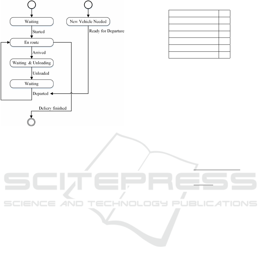
Figure 1: State machine model for individual vehicle.

tions to solution representations. The interaction of

event data and optimization process is explained in

detail in Section 5.

3.2 General Setting and Simulation

Unfortunately, exploring dynamic VRPs in real-

time lacks the availability of compatible benchmarks,

whereas benchmarks for static VRPs are very com-

mon. Hence, one solution to generate an appro-

priate setting for the real-time dynamic VRP is to

adapt static benchmark ﬁles to suit a real-time im-

plementation. Foundations to our work are the well-

known Gehring & Homberger benchmarks for the

static capacitated VRP with time windows (Gehring

and Homberger, 1999).

3.2.1 Description of the Benchmark Files

Besides the maximum number of vehicles K and a

uniform maximum capacity q of each vehicle, the

Gehring & Homberger benchmark ﬁles consist of a

list of N customers. Note, that the ﬁrst customer c

the depot. Each customer can be considered a 7-ary-

tuple containing the values listed in Table 1.

Distances between customers are calculated as

Euclidean distances. Commonly, these benchmarks

suppose that one time unit equals one distance unit.

As this assumption is contradictory to realistic use-

cases, our approach differentiates between time and

distance by using average speed values to calculate

travel times from the given distances.

Table 1: Deﬁnition of customer c

Customer Number i

x-Coordinate x

y-Coordinate y

Demand d

Ready Time e

Due Date l

Service Time f

3.2.2 Introduction of Real-Time

To further enhance the benchmark towards real-time

scenarios, three additional parameters are introduced:

the start time of the delivery period is denoted as t

start

its planned duration is denoted as l

period

and the aver-

age velocity of a vehicle is represented by v. Due to

the fact, that the presented approach runs in system

time, all relevant time parameters must be converted

into milliseconds. Based on these parameters and the

due date of the depot l

, which marks the end of the

delivery period in the static benchmark, two basic co-

efﬁcients can be derived:

time

period

· 60 ·60 · 1000

(1)

distance

v · l

period

(2)

Using these coefﬁcients, time and location data of

the benchmark ﬁles can be adapted to create a real-

time environment. The time and location data of ev-

ery customer c

is adapted as shown below.

i,new

:= x

· f

distance

(3)

i,new

:= e

· f

time

start

(4)

All other relevant parameters are adapted accord-

ingly.

3.2.3 Time-Dependent Travel Times

Time-dependent travel times are crucial as they em-

body changing trafﬁc conditions. Based on the con-

cept of (Ichoua et al., 2003), the calculation period is

divided into discrete, equidistant time intervals with

predeﬁned speed factors. The total travel distance re-

sults as sum of the iteratively calculated partial dis-

tances in each time interval. The travel time can then

be calculated based on the total distance. One advan-

tage of this method is the straightforward implemen-

tation of the FIFO principle, which guarantees, that a

later departure at a speciﬁed destination cannot lead

to a sooner arrival at another.

3.2.4 Dynamic Travel and Service Times

In real-world applications, trafﬁc conditions underlie

dynamic changes due to accidents, construction sites,

congestion and more. To represent this adequately,

we apply a gamma distribution on the time-dependent

speed factors of the model. Speciﬁc parametrizations

then allow the simulation of different trafﬁc scenarios

(Chiang and O. Roberts, 1980).

Additionally, stafﬁng problems and occupied

loading zones e.g. by delay of preceding unloading

processes are only exemplary reasons that cause de-

layed service times in real-world scenarios. For this,

queuing theory proposes the gamma distribution to

generate dynamic service times (Liebermann et al.,

1997). More details on the speciﬁc parametrizations

are provided in Section 6.

3.2.5 Time Windows and Penalty Function

In the Gehring & Homberger benchmarks, each cus-

tomer c

is associated with a time window (e

, l

), in

which the delivery should be started. Time window

violations are taken into account by a penalty func-

tion, which assigns a penalty cost value p

to each

customer. Depending on the end of the time window

and the arrival time s

at customer c

, this is calcu-

lated as follows:

(

penalty

+ c f

penalty

· (s

− l

) if s

> l

0 else.

(5)

In this context, c f

penalty

is a cost factor rating the time

of delay and c

penalty

is the ﬁxed cost part in case of

time window violation.

3.2.6 External Vehicles

For each of the Gehring & Homberger benchmark

ﬁles, a maximum number of vehicles K is speciﬁed.

However, real-time reaction to dynamic events may

require the use of additional vehicles in order to serve

all customer requests, preferably in the given time

windows. Hence, it is possible that K needs to be ex-

ceeded. In this case, our model assumes the possibil-

ity to hire different transportation companies by rent-

ing external vehicles (and drivers) which then carry

out some of the customer requests. Certainly, this im-

plies additional costs. These are assumed to be 20%

higher than the costs in case all customers could be

served by vehicles of the own ﬂeet.

4 ARCHITECTURE

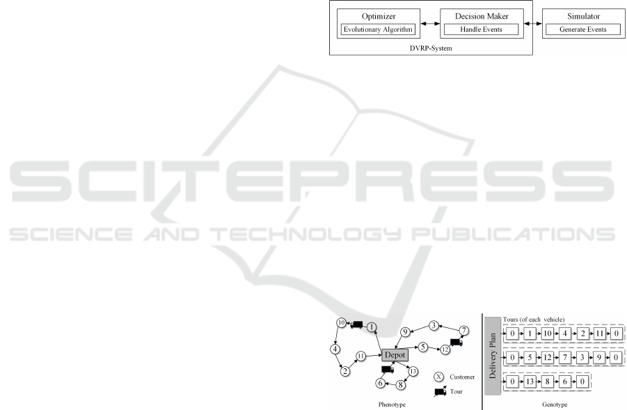
The proposed DVRP-system consists of three main

components, which are reﬂected in Figure 2. The op-

timizer represents the core component of the system

and is responsible for the actual optimization process.

The simulator executes delivery plans in real-time and

produces event data of the simulated ﬂeet. Events for

each vehicle are raised according to the state machine

introduced in Figure 1. The decision maker handles

those events in real-time by updating the information-

base of the optimizer. A further responsibility of the

decision maker is to decide whether it is economically

viable to realize new delivery plans in case a new plan

is proposed by the optimizer.

Figure 2: Architecture of the DVRP-system.

4.1 Optimizer

An evolutionary algorithm is proposed, which en-

hances the hybrid multi-objective evolutionary algo-

rithm (HMOEA) by (Tan et al., 2006). Major parts of

the HMOEA have been adapted, enlarged or substi-

tuted to comply with the requirements of the environ-

mental model. The genotype is encoded as visualized

in Figure 3. According to the representation, a de-

livery plan consists of various tours, which represent

all customers dedicated to a speciﬁc vehicle. A tour

starts and ends at the depot c

. Besides all customers

are represented as integer values.

Figure 3: Encoding of a delivery plan.

The formerly used Pareto ﬁtness ranking of the

HMOEA was replaced by the restricted tournament

selection (RTS) of Harik (Harik, 1995) and com-

bined with a selection method as well as a sim-

ple elitism method. To enable the evaluation of

the distance of different individuals as required in

the RTS, the optimizer uses the Jaccard-Coefﬁcient

in combination with the 2-Gram method (Naumann

and Herschel, 2010). Furthermore, we adopted

the route-exchange-crossover, the three optional mu-

tation methods (split-route-mutation, merge-route-

mutation, partial-swap-mutation), as well as all lo-

cal search heuristics (intra-route-heuristic, lambda-

interchange-heuristic, shortest-path-heuristic) of the

original HMOEA, but adapted them to ﬁt the require-

ments of the real-time model.

4.1.1 Cost Function

To evaluate the ﬁtness of a solution, a newly devel-

oped cost function C

total

was implemented. As costs

are crucial for enterprises and their practical applica-

tion of the VRP, the cost function aggregates three

major cost drivers: distance-dependent costs C

distance

time-dependent costs C

time

and penalty costs C

penalty

For that, the tour time of a vehicle (from start to end

of its delivery) t

is weighted with a time cost factor

c f

time

. Analogously, the tour distance of each vehicle

is weighted by c f

distance

. The total time and dis-

tance costs are then both calculated as sum of the cost

values of all K vehicles. The overall penalty costs

penalty

result from the individual penalty costs p

all N customers.

total

= C

distance

time

penalty

(6)

distance

∑

j=0

(c f

distance

· d

· δ

) (7)

time

∑

j=0

(c f

time

·t

· δ

) (8)

penalty

∑

i=0

(9)

To reﬂect the possibility of hiring external vehi-

cles and the associated extra costs, δ

is introduced

and deﬁned as follows:

(

1.0 if vehicle j is part of ﬂeet,

1.2 if vehicle j is not part of ﬂeet.

(10)

4.2 Simulator

The simulator is responsible for the generation of the

events, which includes the simulation of the dynamic

travel and service times. Aligned to the approach of

(Ichoua et al., 2003), the simulator generates individ-

ual speed factors for each road segment and each time

interval. Based on the simulated speed factors the ac-

tual travel time can be calculated. The dynamic ser-

vice times are simulated by applying the integrated

gamma distribution directly to the updated service

time values of the benchmark ﬁle. The ﬂexible im-

plementation of the simulator facilitates the modular

exchange of different trafﬁc/queuing models, as well

as the integration of real trafﬁc data. Furthermore,

it is possible to substitute the simulator for mobile

devices or vehicle-based on-board devices, using the

same event-based communication protocol.

4.3 Decision Maker

The decision maker represents the interface between

the simulator and the optimizer. It is responsible for

plan updates and the information ﬂow towards the

individual vehicles. For this purpose, the decision

maker continuously compares the current best plan of

the optimizer with the plan currently executed and de-

cides whether a change should be realized. Thereby

an real-time reactivity towards new information, as

well as the alignment of the delivery plan towards the

currently best solution is ensured throughout the en-

tire optimization period.

As all information emerging from the simulator

passes the decision maker, the decision maker is also

responsible for the event handling process. This com-

prises the update of the information base, as well as

the execution of repair routines. These are necessary

in case the individuals of the HMOEA-population

need to be adapted throughout the dynamic optimiza-

tion process.

5 ALGORITHMIC ASPECTS

The communication protocol between the vehicles

and the optimization back-end requires a thorough

deﬁnition of the submitted event data and their

algorithmic consequences. For this purpose, the

decision maker is implemented as interface between

the simulator and the optimizer to handle incoming

events. The tasks of the decision maker can be

divided as follows:

Update of Information-Base

To properly use the incoming information, it has to be

embedded into the information base of the optimizer.

This includes the real-time update of actual and

expected travel/service times as well as the update of

the customer base.

Adaption of Population

Some events also require an update on the population

of the HMOEA to guarantee a consistent set of fea-

sible individuals for the further execution of the opti-

mization process. The importance of this will be ex-

plained subsequently.

5.1 Event Handling

Referring to Figure 1, this section describes all types

of events and their inherent changes to the optimiza-

tion process.

The Arrived-event marks the arrival of a vehicle at

a customer and is handled with a simple routine. The

decision maker processes the received information by

replacing the expected arrival time at the correspond-

ing customer (which was used by the optimizer for

plan calculations until then) by the actual arrival time.

The same procedure is valid for the Unloaded-

event which marks the end of the service period of a

vehicle at a customer. In this case, the decision maker

replaces the expected service time by the actual ser-

vice time.

The Departed-event however requires more so-

phisticated routines. On the one hand the expected

departure time has to be replaced by the actual depar-

ture time. On the other hand the served customer c

old

which the vehicle has departed from, has to be deleted

from the representation. Due to (A) we obtain a ﬁxed

customer c

as a next target for the considered vehi-

cle. This causes the necessity to update the population

of the HMOEA as c

old

has to be deleted from each in-

dividual of the population. Each individual shall now

contain one vehicle heading to c

new

(which means one

tour with c

new

at ﬁrst position).

The same adaptions have to be conducted for the

Started-event, where c

old

is considered as a substitute

for the depot. Additionally, this event marks the be-

ginning of the delivery period and therefore the shift

from static to dynamic optimization.

In case the decision maker proposes the utiliza-

tion of an additional vehicle, the Ready for Depar-

ture-event is triggered and a new vehicle departs at

the depot c

old

heading to a customer c

new

. As a con-

sequence, all individuals of the population have to be

expanded by one vehicle also heading to c

new

(A).

5.2 Repair Routines

To guarantee the individuals of the HMOEA-

population to be feasible at all times, the events

Started and Departed trigger repair mechanisms for

the entire HMOEA-population. Each individual has

to be adapted such that the new customer c

new

is di-

rectly targeted by a vehicle, whereas the served cus-

tomer c

old

is deleted from all individuals. In some

cases, it may be required to relocate several unserved

customers within the individual. Therefore these

customers are transferred to a so-called reloctaion-

list (RL) and later reinserted by a special insertion

method.

5.2.1 Repair Routine for the Departed-Event

In case c

old

and c

new

are scheduled to be served by

the same vehicle, the corresponding tour will be cut

before c

new

, thus making sure that this vehicle serves

new

as next customer. Furthermore, the customers

between c

old

and c

new

are put on the RL (Figure 4).

Figure 4: Repair routine for the Departed-event (case 1).

If c

new

is contained in a different tour than c

old

, all

customers of the tour that contains c

old

will be trans-

ferred to the RL. The customers of the tour containing

new

will be divided as visualized in Figure 5. This en-

sures that the considered vehicle keeps on heading to

the customer that it is targeting (customer 6 in the ex-

ample) while the vehicle, whose tour contained c

old

is now targeting c

new

Figure 5: Repair routine for the Departed-event (case 2).

Repair Routine in Pseudo-Code:

Find tour containing c_old;

Delete c_old;

if(c_new is contained in same vehicle)

Put customers before c_new on RL;

Delete customers before c_new;

else

Delete last customer (depot);

Put remaining customers on RL;

Find tour containing c_new;

Divide tour at c_new;

Replace vehicle that contained c_old;

5.2.2 Repair Routine for the Started-Event

In the case of the Started-event all scheduled vehicles

leave the depot at the beginning of the delivery pe-

riod. Thereby, each vehicle gets assigned a ﬁxed ﬁrst

customer (c

new

). In the following, the set containing

these customers is denoted S. To update the individu-

als of the HMOEA-population, in a ﬁrst step the depot

at ﬁrst position of each vehicle’s tour is deleted. Sub-

sequently, for each tour it is checked whether its ﬁrst

customer is contained in S. If so, this tour remains un-

changed and the corresponding customer gets deleted

from S. In the other case, the vehicle is put to a recom-

bination list. In a third step, the remaining customers

Figure 6: Repair routine for the Started-event.

in S are deleted from the tour. Finally the customers

in S are recombined with the remaining tours in a cost

efﬁcient way to create a new individual that is fea-

sible. For a short example on this repair routine see

Figure 6.

In case no feasible way of recombination is found,

customers of the remaining vehicle representations

are transferred step by step to the relocation list

until a feasible recombination is obtained. After this

procedure, the customers of the RL are reinserted

using the insertion method.

Repair Routine in Pseudo-Code:

Delete first customer of each individual;

for (each tour)

if (first customer of tour is in S)

Delete customer from tour;

Delete customer from S;

else

Put tour on recombination list;

end

Delete customers in S from tours;

Recombine customers in S with remaining tours

of recombination list;

while (no feasible combination found)

Put random customer (not contained in S)

to relocation list;

Recombine customers in S with remaining

tours of recombination list;

end

5.2.3 Insertion Method

The insertion method is in charge of the reinsertion of

the customers that were transferred to the relocation

list by the repair routines. To minimize the loss of

optimization knowledge, it is aspired to maintain

the major parts of the customer-sequence. There-

fore, this method randomly inserts (and instantly

deletes) the ﬁrst customer of the RL at a predeﬁned

number of positions in the genotype and calculates

the corresponding cost value. Subsequently, the

customer is inserted at the position, that causes

minimal additional costs. If no feasible insertion

position is found, a new vehicle is required to serve

this customer. Thereafter, all following customers

are inserted and deleted from the RL as long as there

is no violation to the capacity limitation. In case of

violation this procedure starts anew.

Insertion Method in Pseudo-Code:

while(customers contained in RL)

for (counter < number of attempts)

Insert first customer of RL at random

position in genotype;

if (feasible)

Evaluate cost function;

Delete first customer from genotype;

Counter++;

end

if (feasible position found)

Insert first customer at best position;

else

Insert customer in new vehicle;

while (no violation to capacity)

Insert following customers from RL;

end

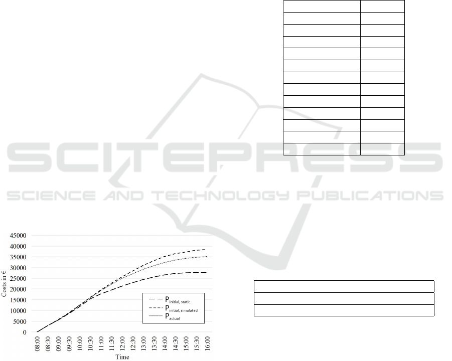
6 EVALUATION

The aim of this chapter is a holistic evaluation of

the repair routines. As a ﬁrst step, this paper vali-

dates their general functionality and impact towards

different dynamic problem instances. Future research

should focus on a detailed analysis and the further en-

hancement of the approach. In order to evaluate the

performance of the dynamic optimization, the evalu-

ation concept is based on the comparison of the ini-

tial delivery plan and the actual plan. The actual plan

actual

results from the initial delivery plan P

initial,static

by constant changes through the continuous reactions

of the optimization back-end to the dynamic environ-

ment, whereas the initial plan is the result of the static

optimization at the beginning of the delivery period.

Assuming this delivery plan is exposed to the dy-

namic events without online re-optimization, Figure

7 shows the respective cost as P

initial,simulated

. To en-

sure the comparability of P

initial,simulated

with P

actual

it is crucial to use the same underlying trafﬁc condi-

tions and service times. Figure 7 shows the typical

progression of the cost functions of the three consid-

ered plans.

Figure 7: Typical progression of the cost functions.

6.1 Test Setup

The real-time test setup employs the C101 instances

of the Gehring & Homberger benchmarks for 200,

400, 600, 800 and 1000 customers. Each of these

instances was simulated using three different shifted

gamma distributions. Every combination of the test

instances and the gamma distributions was repeated

ten times with different random seeds, which resulted

in 150 test runs. All instances model an entire real-

time distribution period starting the static optimiza-

tion at 8.00 pm the day before the actual delivery took

place. Dynamic optimization starts with the begin-

ning of the distribution period at 8.00 am and contin-

ues until 4.00 pm. All relevant parameters used in the

test setup are shown in Table 2. For a detailed deﬁ-

nition of the genetic parameters, please refer to (Tan

et al., 2006).

Table 2: Test parameters.

Crossover-rate 0.7

Mutation-rate 1.0

Elastic-rate 0.5

Squeeze-rate 0.7

Population-size 20

Elitism-quantity 3

c f

distance

1e/km

c f

time

60e/h

c f

penalty

50e/h

base

100e

start

8:00 am

l 8h

v 70km/h

The focus is set on evaluating different trafﬁc con-

ditions and their impact on the optimization process.

Hence, one single parameter setting was used for the

simulation of the dynamic service times. The service

time is reﬂected by the gamma distribution (1, 0.25)

which is shifted by 0.75. The three gamma distribu-

tions, which were used for the simulation of the dy-

namic service times are shown in Table 3 .

Table 3: Parameter for the gamma distribution.

Distribution 1: Γ(1, 0.25), Shift: 0.75

Distribution 2: Γ(1, 0.50), Shift: 0.5

Distribution 3: Γ(1, 0.75), Shift: 0.25

The distribution parameters have been chosen fol-

lowing the approach of (Russell and Urban, 2008)

where the gamma distribution was applied to model

dynamic travel times. The expected value equals 1 in

all cases.

6.2 Test Evaluation

The ﬁnal average results of all 150 test instances

grouped by the number of customers are shown in Ta-

ble 4. The results indicate the percentage, as well as

the total deviation of P

actual

from P

initial,simulated

. In

total, an average saving of 6.58% in the overall costs

Table 4: Test results on different instances of the adapted Gehring & Homberger C101 benchmark ﬁles.

could be achieved. The overall saving is primarily

caused by a signiﬁcant reduction of the penalty costs

and usually results in an increase of the distance and

time values. As shown in the table, the increase in the

distance and time values seems to correlate with the

number of processed customers. The instances with

less customers generally indicate a higher increase

in the corresponding values, than the instances with

more customers. The number of additional vehicles

is also increasing by 0.92% to 3.92% which means

up to three additional vehicles in average. However,

there was no test instance in which the number of

vehicles exceeded the maximum ﬂeet size K of the

C101 Gehring & Homberger benchmarks. This im-

plies that no external vehicle was needed in all test

instances. The percentual reduction of time window

violations is decreasing with the number of processed

customers, whereas the total number reaches its peak

at the test instances with 600 customers. As the num-

ber of time window violations is directly affecting the

penalty costs, similar characteristics are reﬂected in

these results. The achieved results indicate a reli-

able performance of the implemented repair routines

in various test settings, by achieving overall average

savings between 4.98% and 7.66%.

7 CONCLUSION

This paper proposed an approach to real-time ﬂeet

event handling for the DVRP based on evolutionary

computation. In contrast to other approaches, the sys-

tem allows for rapid responses to dynamic events and

processes dynamic travel times as well as dynamic

service times. The system is able to simulate real-time

delivery periods lasting up to one day and is designed

for further expansion like the inclusion of GPS-data

or real event data. With the two newly developed

repair routines, new innovative methods were imple-

mented to ensure a continuous creation of feasible de-

livery plans. The system runs a time-dependent travel

time model and optimizes the total costs of the deliv-

ery plan including penalty costs for delayed delivery.

In empirical studies the system and its repair routines

could be validated in different test scenarios. Further-

more, the DVRP-system led to cost savings between

4.98% and 7.66% in all test scenarios.

8 FUTURE WORK

The ﬂexible and modular system implementation, al-

lows for easy extension and adaption. Even the sub-

stitution of essential parts such as the simulator is pos-

sible with little effort. This is enabled by a smart and

lightweight system architecture with a clearly struc-

tured message exchange protocol between the system

components.Therefore, the system could be extended

by additional dynamic aspects such as dynamic cus-

tomer orders. In order to test the system in a real-

life scenario, the simulator is projected to be substi-

tuted and replaced by mobile devices and/or be con-

nected to on-board vehicle-based systems. Such alter-

nate edge devices would then be responsible for the

information (event) transfer towards the optimization

back-end. The adaption of the current system would

require very little effort only. As a long-term goal, it

is aspired to include GPS-data. Besides these struc-

tural adaptions of the system, it is crucial for further

development to enlarge the test evaluation towards ad-

ditional benchmark tests. Especially, more restrictive

settings considering the ﬂeet size would be preferable

to evaluate the concept of external vehicles and the

inﬂuence of the associated extra costs δ

. Further re-

search focuses on a detailed analysis of repair routines

and their impact on the optimization process. Ad-

ditionally, existing optimization algorithms like Ant

Colony Optimization or Particle Swarm Optimization

and other solution strategies for the DVRP (Psaraftis

et al., 2016) need to be adapted to the proposed dy-

namic real-time VRP-environment to ensure compa-

rability. The gathered insights can then be used to

gain optimization performance.

REFERENCES

AbdAllah, A. M. F., Essam, D. L., and Sarker, R. A. (2017).

On solving periodic re-optimization dynamic vehicle

routing problems. Applied Soft Computing, 55:1–12.

Barkaoui, M. and Gendreau, M. (2013). An adaptive

evolutionary approach for real-time vehicle routing

and dispatching. Computers & Operations Research,

40(7):1766–1776.

Bektas, T., Repoussis, P., and Tarantilis, C. (2014). Dy-

namic vehicle routing problems. In Toth, P. and Vigo,

D., editors, Vehicle routing, MOS-SIAM series on op-

timization, pages 299–347. Society for Industrial and

Applied Mathematics and Mathematical Optimization

Society, Philadelphia.

Branke, J., Middendorf, M., Noeth, G., and Dessouky, M.

(2005). Waiting strategies for dynamic vehicle rout-

ing. Transportation Science, 39(3):298–312.

Chiang, Y.-S. and O. Roberts, P. (1980). A note on transit

time and reliability for regular-route trucking. Trans-

portation Research Part B: Methodological, 14(1-

2):59–65.

eput, J.-C., Hajjam, A., Koukam, A., and Kuhn, O.

(2012). Self-organizing maps in population based

metaheuristic to the dynamic vehicle routing problem.

Journal of Combinatorial Optimization, 24(4):437–

458.

Elhassania, M., Jaouad, B., and Ahmed, E. A. (2014). Solv-

ing the dynamic vehicle routing problem using ge-

netic algorithms. In 2014 International Conference on

Logistics and Operations Management (GOL), pages

62–69.

Gan, Z., Tao, L., and Ying, Q. (2013). Automated guide ve-

hicles dynamic scheduling based on annealing genetic

algorithm. Indonesian Journal of Electrical Engineer-

ing and Computer Science, 11(5):2508–2515.

Gehring, H. and Homberger, J. (1999). A parallel hy-

brid evolutionary metaheuristic for the vehicle rout-

ing problem with time windows: Jyv

askyl

a, ﬁnnland.

In Miettinen, K., M

akel

a, M., and Toivanen, J., ed-

itors, Proceedings of EU-ROGEN99, pages 57–64,

Jyv

askyl

a, Finnland.

Ghannadpour, S. F., Noori, S., and Tavakkoli-Moghaddam,

R. (2013). Multiobjective dynamic vehicle routing

problem with fuzzy travel times and customers’ sat-

isfaction in supply chain management. IEEE Trans-

actions on Engineering Management, 60(4):777–790.

Ghannadpour, S. F., Noori, S., Tavakkoli-Moghaddam, R.,

and Ghoseiri, K. (2014). A multi-objective dynamic

vehicle routing problem with fuzzy time windows:

Model, solution and application. Applied Soft Com-

puting, 14:504–527.

Haghani, A. and Jung, S. (2005). A dynamic vehicle routing

problem with time-dependent travel times. Computers

& Operations Research, 32(11):2959–2986.

Hanshar, F. T. and Ombuki-Berman, B. M. (2007). Dy-

namic vehicle routing using genetic algorithms. Ap-

plied Intelligence, 27(1):89–99.

Harik, G. (1995). Finding multimodal solutions using re-

stricted tournament selection. In Eshelman, L. J., edi-

tor, Proceedings of the Sixth International Conference

on Genetic Algorithms, pages 24–31. M. Kaufman,

San Francisco, Calif.

Ichoua, S., Gendreau, M., and Potvin, J.-Y. (2003). Vehicle

dispatching with time-dependent travel times. Euro-

pean Journal of Operational Research, 144(2):379–

396.

Liebermann, G. J., Hillier, F. S., Fackler, M., Bauer,

G., Honold, G., Michels, K.-N., Rehklau, U.,

and Weigert, M. (1997). Operations Research:

Einf

uhrung. Internationale Standardlehrb

ucher der

Wirtschafts- und Sozialwissenschaften. De Gruyter

Oldenbourg, M

unchen, 5. auﬂ. edition.

Naumann, F. and Herschel, M. (2010). An introduction to

duplicate detection, volume #3 of Synthesis lectures

on data management. Morgan & Claypool Publishers,

San Rafael, Calif.

Pillac, V., Gendreau, M., Gu

eret, C., and Medaglia, A. L.

(2013). A review of dynamic vehicle routing prob-

lems. European Journal of Operational Research,

225(1):1–11.

Psaraftis, H. N., Wen, M., and Kontovas, C. A. (2016). Dy-

namic vehicle routing problems: Three decades and

counting. Networks, 67(1):3–31.

Ritzinger, U., Puchinger, J., and Hartl, R. F. (2015). A sur-

vey on dynamic and stochastic vehicle routing prob-

lems. International Journal of Production Research,

54(1):215–231.

Russell, R. A. and Urban, T. L. (2008). Vehicle routing with

soft time windows and erlang travel times. Journal of

the Operational Research Society, 59(9):1220–1228.

Tan, K. C., Chew, Y. H., and Lee, L. H. (2006). A hybrid

multiobjective evolutionary algorithm for solving ve-

hicle routing problem with time windows. Computa-

tional Optimization and Applications, 34(1):115–151.

Taniguchi, E. and Shimamoto, H. (2004). Intelligent trans-

portation system based dynamic vehicle routing and

scheduling with variable travel times. Transporta-

tion Research Part C: Emerging Technologies, 12(3-

4):235–250.