Hierarchy Influenced Differential Evolution: A Motor Operation
Inspired Approach
Shubham Dokania, Ayush Chopra, Feroz Ahmad and Anil Singh Parihar
Delhi Technological University, New Delhi, India
Keywords:
Differential Evolution, Metaheuristics, Continuous Optimization, Hierarchical Influence.
Abstract:
Operational maturity of biological control systems have fuelled the inspiration for a large number of mathe-
matical and logical models for control, automation and optimisation. The human brain represents the most
sophisticated control architecture known to us and is a central motivation for several research attempts across
various domains. In the present work, we introduce an algorithm for mathematical optimisation that derives its
intuition from the hierarchical and distributed operations of the human motor system. The system comprises
global leaders, local leaders and an effector population that adapt dynamically to attain global optimisation via
a feedback mechanism coupled with the structural hierarchy. The hierarchical system operation is distributed
into local control for movement and global controllers that facilitate gross motion and decision making. We
present our algorithm as a variant of the classical Differential Evolution algorithm, introducing a hierarchical
crossover operation. The discussed approach is tested exhaustively on standard test functions as well as the
CEC 2017 benchmark. Our algorithm significantly outperforms various standard algorithms as well as their
popular variants as discussed in the results.
1 INTRODUCTION
Evolutionary algorithms are classified as meta-
heuristic search algorithms, where possible solution
elements span the n-dimensional search space to find
the global optimum solution. Over the years, nat-
ural phenomena and biological processes have laid
the foundation for several algorithms for control and
optimization that have highlighted their applicabil-
ity in solving intricate optimization problems. For
instance, at the cellular level in the E.Coli Bac-
terium, there is sensing and locomotion involved in
seeking nourishment and avoiding harmful chemi-
cals. These behavioral characteristics fuelled the in-
spiration for the Bacterial Foraging Optimization al-
gorithm (Passino, 2002)(Onwubolu and Babu, 2013).
Particle Swarm Optimization (Kennedy and Eberhart,
1995) is a swarm intelligence algorithm based on be-
havior of birds and fishes that models these particles
as they traverse an n-dimensional search space and
share information in order to obtain global optimum.
From a biological control point, the human brain
represents one of the most advanced architectures and
several research attempts seek to mimic its functional
accuracy, precision and efficiency. The brain func-
tion activities can be broadly classified into 2 cate-
gories: sensory and motor operations. Sensory corti-
cal functions inspired the concept of neural networks
that are being scaled successfully in deep learning to
solve vast amount of problems.
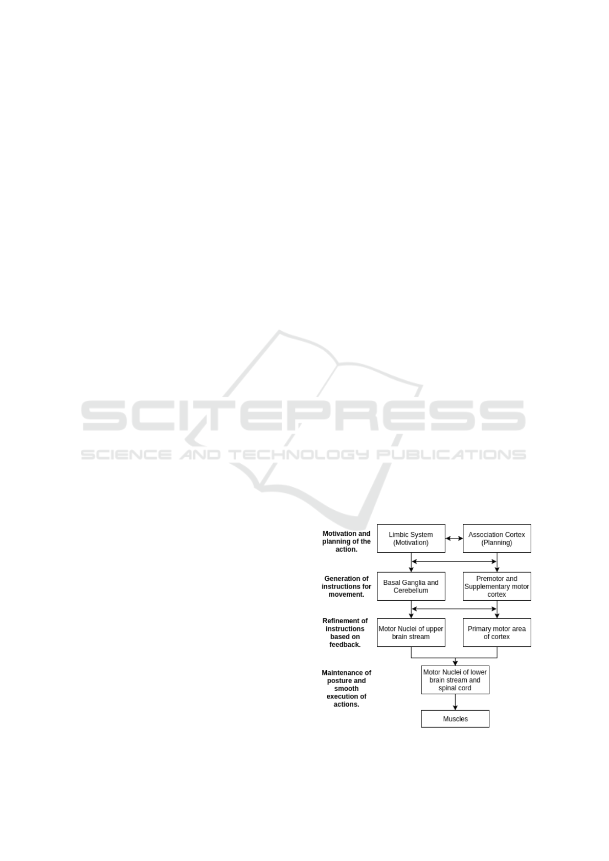
The human motor function represents a distributed
neural and hierarchical control system. It can be clas-
sified as having local control functions for movement
Figure 1: Hierarchy of Motor Control in Humans.
Dokania S., Chopra A., Ahmad F. and Parihar A.
Hierarchy Influenced Differential Evolution: A Motor Operation Inspired Approach.
DOI: 10.5220/0006490302070214
In Proceedings of the 9th International Joint Conference on Computational Intelligence (IJCCI 2017), pages 207-214
ISBN: 978-989-758-274-5
Copyright
c
 2017 by SCITEPRESS – Science and Technology Publications, Lda. All rights reserved

as well as higher level controllers for gross motion
and decision making. The execution of motor op-
eration involves distributed brain structures at differ-
ent levels of hierarchy. These include the pre-frontal
cortex, motor cortex, spinal cord, anterior horn cells
etc (Shaw et al., 1982). For executing an action se-
quence, a sequence of actions is implemented by a
string of subsequences of actions each implemented
in a different part of the body. The operational struc-
ture has been depicted in Figure 1(Passino, 2005).
For optimality of actions, neurons act in unison. The
neurons in the motor cortex act like global leaders
and send inhibitory or facilitatory influence over ante-
rior horn cells, the local leaders, located in the spinal
cord(Shaw et al., 1982). These local leaders are con-
nected to muscle fibers, the effectors, through a pe-
ripheral nerve and neuromuscular junction. Efficient
execution of task requires feedback based facilitation
and inhibition of the effectors over the anterior horn
cells. These sequence of operations realise the opti-
mal convergence of the system leading to smooth mo-
tor execution.
The present work introduces an algorithm mod-
elled intuitively on the distributed and hierarchical op-
eration of the brain motor function.
The Classical DE Algorithm (Storn and Price,
1995), proposed by Storn and Price has been hailed as
one of the premier evolutionary algorithms, owing to
its simple yet effective structure(Das and Suganthan,
2011). However, in recent times, it has been criticized
for its slow convergence rate and inability to effec-
tively optimize multimodal composite functions(Das
and Suganthan, 2011). This work focusses on sup-
plementing the algorithm’s performance through the
introduction of hierarchical influence in the pipeline.
The architecture enables the algorithm to control the
flow of agents through the cummulative effect of
global and local leaders in the hierarchy.
The proposed approach, Hierarchy Influenced Differ-
ential Evolution (HIDE), has been subjected to ex-
haustive analysis on the hybrid and composite ob-
jective functions of the CEC 2017 benchmark(Awad
et al., 2016). Comparison with the classical DE algo-
rithm and its other popular variants including JADE
and PSODE (Zhang and Sanderson, 2009) highlights
the particular viability of the schemed approach in
solving complex optimization tasks. We show that
even with fixed parameters, HIDE is able to outper-
form adaptive architectures such as JADE by a re-
spectable margin, as discussed in the result sections.
2 CLASSICAL DIFFERENTIAL
EVOLUTION
Figure 2: Motion planning of individuals in DE on two di-
mensional example of objective function.
The classical Differential Evolution (DE) algorithm
is a population-based global optimization algorithm,
utilizing a crossover and mutation approach to gen-
erate new individuals in the population for achieving
optimum solutions(Das and Suganthan, 2011). For
each individual x
i
that belongs to the population for
generation G, DE randomly samples three individu-
als from the population namely x
r1,G
, x
r2,G
and x
r3,G
.
Employing these randomly chosen points, a new in-
dividual trial vector, v
i
, is generated using equation
(1):
v
i
= x
r1,G
+ F(x
r2,G
− x
r3,G
) (1)
Where, F is called the differential weight (Usually
lies between [0,1]).
To obtain the updated position of the individual,
a crossover operation is implemented between x
i,G
and v
i
, controlled by the parameter CR called the
crossover probability. The value for CR always lies
between [0,1].
3 HIERARCHY INFLUENCED
DIFFERENTIAL EVOLUTION
Taking inspiration from the human motor system, we
model the hierarchical motor operations in our op-
timization agents, where we define a global leader
which influences the action of several distributed lo-
cal leaders and the particle agents which act as the
effectors. The global leader is analogous to the de-
cision making and planning section in the motor sys-
tem hierarchy whilst, the local leaders correspond to
motion generators acting under the influence of the
global leader.
The position of each particle in the population
is affected by the influence of global leader and lo-

cal leaders, while also being affected by a randomly
chosen particle from the population to induce some
stochasticity in the optimization pipeline. We first
model the influence of the global leader on the lo-
cal leaders and the influences of the local leaders on
each population element using equation (3) and (4).
We introduce a hierarchical crossover between the
two influencing equations governed by a hierarchical
crossover parameter HC.
Analogously to the brain motor operation as de-
picted in Figure 1, the update of particle positions re-
quires generating feedback for the leaders as a part of
the optimization procedure, and hence the local lead-
ers and the global leader are updated based on their
objective function value generated from the perturba-
tions in population particles. This series of events
comprise of one optimization pass (one generation
step). On execution of several optimization passes as
Algorithm 1: Hierarchy Influenced Differential Evolution.
1: procedure START
2: Initialize parameters (HC, F, P, N
l
, NP).
3: Generate initial global leader g
L
as a random
point.
4: Generate N
l
local leader points around g
L
global leader.
5: Generate NP points for population P around
the local leaders using a Normal distribution with
identity covariance.
6: while Termination criteria is not met do
7: for each individual x
i,G
in P do
8: Determine the corresponding local
leader x
L
i
,G
from the set of all local leader based
on nearest position.
9: Let u = 0 be an empty vector.
10: Let G and G
t
be the current generation
and total generations of the procedure.
11: if G < (HC ∗ G
t
) then
12: u
i
= E
g
from (3).
13: else
14: u
i
= E
l
from (4).
15: end if
16: x
0
i
= BinomialCrossover(u
i
, x
i,G
, CR)
17: if f (x
0
i
) < f (x
i,G
) then
18: Replace x
i,G
with x
0
i
in the next
generation.
19: end if
20: end for
21: Alter local leaders in each population
cluster based on objective function value.
22: Compute updated global leader g
L
.
23: end while
24: end procedure
described, the system is able to converge to an opti-
mal configuration, analogous to the successful execu-
tion of the required task as shown in the final steps of
Figure 1.
For each particle x
i,G
, i = 0,1,2,...NP −1 for gen-
eration G, the trial vector x
0
i
of the particle, is governed
by the hierarchical crossover operation and a mutation
operation as follows :
u
i
=

E
g
, i f G < HC ∗ G
t
E
l
, otherwise
(2)
E
g
= g
L
+ F(x
L
i
,G
− x
r,G
) (3)
E
l
= x
L
i
,G
+ F(x
i,G
− x
r,G
) (4)
for each dimension j of x
j,i,G
:
x
0
j,i
=

x
j,i,G
i f rand(0,1) < HC
u
j,i
otherwise
(5)
x
i,G+1
=

x
0
i,G
, i f f (x
0
i,G
) < f (x
i,G
)
x
i,G
, otherwise
(6)
where,
G
t
is the total number of generations,
x
i,G+1
is the vector position of x
i,G
for next generation
F is factor responsible for amplification of differen-
tial variation,
f is the objective function,
x
i,G
is the current position of the individual for
generation G,
u
i
is the intermediate trial vector of the current
individual,
E
g
represents the global and local leader interaction,
E
l
represents the local leader and effector interaction,
g
L
is the global leader for generation G,
x
L
i
,G
is the position of the local leader for current
individual,
Algorithm 2: Binomial Crossover(u, x, CR).
1: procedure START
2: Let x
0
= 0 be an empty vector.
3: Select a random integer k = irand({1,2,...,d});
where d = number of dimensions
4: for each dimension j do
5: if random(0,1) < CR or j == k then
6: Set x
0
j
= u
j
7: else
8: Set x
0
j
= x
j
9: end if
10: end for
11: end procedure

Figure 3: Hierarchical Decisive Motion planning of indi-
viduals in HIDE on two dimensional example of objective
function. The position vectors resulting from the influence
of global leader and local leaders are both represented as
E
g
and E
l
on the contour of a two dimensional objective
function.
x
r,G
ε P ; r ε [0,1,.. NP-1]
x
0
j,i
is the trial vector
x
r,G
is randomly chosen particle from the popula-
tion to induce stochasticity. The hierarchical opera-
tion is affected by the global leader g
L
and the local
leader x
L
i
,G
through the parametric equations (3) and
(4). Switching between the two is governed by the
hierarchical crossover parameter HC.
3.1 Hierarchical Crossover
Convergence trend in HIDE is largely pivoted about
(3) and (4), which in unison, lend a hierarchical struc-
ture to the algorithm. A successful optimization algo-
rithm involves establishing a trade-off between explo-
ration and exploitation. Achieving global optimiza-
tion can be visualized as collaboration of two forces,
exploration over a larger subspace followed by inten-
sive exploitation over the resulting search space gov-
erned by clusters. Phase 1, involving (3) is marked
by the interaction between the global and local lead-
ers representing decision planning and facilitation of
gross motion. This is followed by phase 2, involving
(4) wherein the local leaders interact with and guide
their effector population to control intricate motion
over the constraint subspace to achieve smooth con-
vergence. Robust covergence necessitates an optimal
transition from phase 1 to phase 2 in the hierarchy.
This hierarchical transition is characterized by our
proposed parameter, HC. The value of HC belongs to
[0,1]. An optimal value for HC was observed experi-
mentally to lie about one-quarter. For the purpose of
our experiments, we have fixed HC to be 0.27. Thus,
this defines a deterministic cut after 27% of the total
generation budget. The crossover probability defined
here was observed to be mostly 50% smaller in com-
parison to other DE variants.
The HIDE algorithm achieves a performance im-
provement in the early optimization phase (G ¡ HC ∗
G
t
) by replacing clusters of the initially generated
candidate solutions with the locally best. This strat-
egy rules out a number of mutation vectors that are
more unfavorable in terms of performance gain. Ad-
ditionally, by focusing on mutants of the globally best
candidate solution the search space is explored rather
quickly during this phase. After the population ad-
vances to HC ∗G
t
generations, the algorithm changes
its reference point (the trial vector) to the locally best
candidate solutions of a certain cluster. That is, hav-
ing approached a closer distance from the optimal,
the algorithm is able to exploit the search space. Our
proposition is complemented by the observations in
our results section wherein we significantly outper-
form several popular algorithms on involved multi-
modal hybrid and composite functions in higher di-
mensions.
4 RESULTS AND DISCUSSIONS
All evaluations were performed using Python 2.7.12
with Scipy(Oliphant, 2007) and Numpy(Van Der Walt
et al., 2011) for numerical computations and Mat-
plotlib (Hunter, 2007) package for graphical repre-
sentation of the result data. This section is divided
into two sub-sections: Section A provides description
about the problem set used for analysis of algorith-
mic efficiency and accuracy, and section B comprises
of tabular and graphical data to reinforce the claim of
superiority of the proposed approach.
Table 1: Algorithm Parameter Settings used for compari-
sion.
Algorithm Parameter Value
DE
F 0.5
CR 0.9
PSODE
w 0.7298
φ
p
1.49618
φ
g
1.49618
F r ε [0.9,1.0)
CR r ε [0.95,1.0)
JADE
p 0.05
c 0.1
HIDE
HC 0.27
F 0.48
CR 0.9
N
l
5

Table 2: Objective Function Value for Dimension: 30.
f
id
DE JADE PSO-DE HIDE
best mean best mean best mean best mean
f
1
100.001508 4334.43848 100.001338 100.056201 364.295574 4236.36321 100.0 100.0
f
2
40412441.0 5.1296e+19 200.0 1535352368 332899.0 9.59068e+11 200.0 159855.5
f
3
17926.8728 22131.5427 69304.9261 74080.7004 15792.5475 21683.2090 3679.81159 8999.94726
f
4
481.255055 519.422652 403.633939 442.206911 468.341175 479.341966 400.004163 443.016156
f
5
689.041352 737.79326 667.50756 735.204027 715.904429 746.548906 685.40454 738.842184
f
6
643.626307 652.582714 651.39169 655.142819 642.724237 655.106996 644.701241 652.002395
f
7
883.347367 962.591129 779.907693 818.344111 790.014281 854.285524 812.923573 856.90477
f
8
923.37426 967.251501 931.500175 957.362003 915.414882 960.486239 930.288539 964.11663
f
9
5652.48396 7878.78144 4953.05469 5146.60095 6018.41719 9042.41018 4003.11807 4734.98436
f
10
3596.63104 4536.98976 4012.72329 4204.18969 3934.60671 4863.74111 3793.78177 4346.74134
f
11
1162.40596 1184.63401 1152.74853 1174.58813 1165.14499 1189.17178 1149.74849 1171.13041
f
12
56679.4351 317650.613 24821.1717 58930.0902 10221.0774 161046.055 9208.28924 41947.2226
f
13
3002.02949 18794.8359 4276.90774 13775.8162 3871.27983 10612.2635 1664.06241 2453.60697
f
14
1773.18079 5502.16038 1496.21986 42868.9158 1555.45276 4029.80853 1462.92685 1504.19151
f
15
1860.43566 2484.68996 1688.05046 2222.67432 1651.74747 2223.06054 1611.07440 1852.66177
f
16
2517.43962 2827.00496 2344.19818 2621.61868 2239.24272 2664.11466 2298.04196 2691.67481
f
17
2321.17594 2604.52977 2062.89802 2546.99559 2107.43677 2457.34021 1820.80664 2418.72383
f
18
38987.2824 94156.3285 11841.6081 184888.162 62294.8532 118430.289 12578.0037 23024.1119
f
19
2043.46988 3010.23537 1959.71819 2156.95787 3049.52231 6840.40839 1949.27171 1987.86676
f
20
2625.53915 2864.83261 2706.31444 2805.60006 2619.99649 2895.10724 2753.80621 2966.03579
f
21
2412.08175 2504.77777 2414.52134 2456.71898 2431.74029 2478.84135 2200.0 2442.73431
f
22
2300.48179 5655.56932 2300.0 4157.69878 2307.72135 6811.06916 2300.00998 6795.24842
f
23
3050.65450 3572.96506 2772.00202 2946.74932 2764.92246 3199.87436 2883.27689 3543.83934
f
24
3104.62369 3290.69875 2891.55764 2965.22556 2911.63347 2983.77293 2500.0 2940.75997
f
25
2916.18065 2946.71175 2875.10684 2881.09138 2875.49884 2889.94367 2874.17111 2877.48490
f
26
4043.69140 6756.3724 2900.0 3266.51098 2800.00780 3273.12876 2900.0 3298.49053
f
27
3200.00585 3998.87649 3145.81035 3189.82261 3145.42523 3639.63413 3132.81628 3284.28897
f
28
3290.74402 3326.26398 3100.0 3131.02731 3195.48683 3225.59405 3100.0 3115.50582
f
29
3720.31459 4115.18580 3305.31013 3626.88755 3535.95229 3867.59306 3352.84505 3709.10237
f
30
3359.03076 3900.82666 3263.49653 3749.61072 3312.63502 3524.71447 3298.70464 3421.71532
w/t/l 2/0/28 0/0/30 8/2/20 11/0/19 4/0/26 1/0/29 15/2/13 17/0/13
Table 3: Objective Function Value for Dimension: 50.
f
id
DE JADE PSO-DE HIDE
best mean best mean best mean best mean
f
1
5884574.87 367294248.5 136.072384 3708.75086 5811.21899 154233.646 106.072862 3665.41927
f
2
4.7181e+24 3.3649e+44 2635725.0 5.0237e+26 2.2121e+19 2.5445e+23 2.2799e+17 1.0072e+31
f
3
45520.9663 62237.2968 143481.793 156166.762 52308.4274 64435.2406 44613.2999 58182.8373
f
4
574.400328 801.384952 418.580378 470.113207 477.080964 574.528479 400.005049 447.775413
f
5
816.394775 843.258843 809.89948 834.13126 778.59312 831.066954 791.405194 830.218472
f
6
652.54191 655.794152 633.21788 654.893828 653.291336 658.183613 645.25633 656.060597
f
7
1109.02123 1263.03848 889.036574 944.90319 915.153525 1047.43879 989.957862 1186.2487
f
8
1139.27892 1175.8931 1118.3391 1144.60474 1092.62639 1159.03235 1100.4760 1168.5299
f
9
22196.3878 29218.7759 11958.2800 13174.6623 24753.0405 32233.9545 10251.4763 14752.7168
f
10
6228.49289 7289.18367 6054.70769 6833.30631 6207.79530 7055.59523 6050.43437 6609.80456
f
11
1170.85860 1258.51763 1202.69485 1232.20426 1206.15456 1252.93954 1156.4396 1205.2544
f
12
677263.079 16987989.9 74784.6159 530814.648 584300.698 3448448.79 126908.215 494471.075
f
13
6005.53530 16893.94992 2041.48812 4332.5945 1572.25297 4301.82960 1484.76179 7760.05613
f
14
38490.5323 174367.450 2466.04705 238838.470 16327.4231 67939.0002 2967.8184 26290.3161
f
15
2278.14122 26989.2555 13553.0418 25636.7696 3443.58734 9167.26709 1938.20040 14976.7218
f
16
2722.02601 3176.91690 2345.40070 2916.56101 2521.93881 3146.04527 2436.44933 2978.37746
f
17
2799.94977 3289.61565 2568.38357 2907.86927 2887.28110 3236.95792 2561.37030 2874.96503
f
18
264037.125 872072.477 36176.5867 113941.317 26965.2851 114846.121 260540.781 536454.326
f
19
10051.9124 20380.2571 2089.17225 7763.17234 9905.85082 16555.7569 2013.12690 3609.25896
f
20
2950.92319 3274.33401 3041.81309 3113.28946 2991.58929 3361.82394 2495.03177 3080.13747
f
21
2596.7256 2689.68836 2526.19089 2597.6771 2555.8788 2642.38159 2447.75827 2570.91101
f
22
9713.99324 10803.6537 10759.5967 11032.8809 8918.43626 10465.0224 8181.4460 9755.0703
f
23
3451.10494 4200.17442 2971.16064 3237.77866 2977.55496 3490.63975 2851.65025 3162.31362
f
24
3434.46502 3682.84670 3103.95517 3185.38267 3036.79960 3158.33050s 3136.92774 3284.65609
f
25
3141.14488 3292.30344 2931.16295 2962.47175 2931.92695 3008.89535 2931.14231 2954.76783
f
26
4906.13284 7989.49096 2900.0 3346.87403 2900.44189 3653.75774 2900.0 3262.66849
f
27
3200.01070 3792.64558 3143.03805 3184.64635 3158.17823 3397.13032 3141.01087 3176.01152
f
28
3300.01082 3431.57091 3240.72586 3288.25303 3263.20714 3300.25760 3243.63199 3294.37323
f
29
3812.47551 4605.34953 3533.94574 3956.83524 3955.32453 4364.18129 3653.67555 3966.47195
f
30
3673.71196 5813.17375 3916.72571 4869.08933 3730.30935 5143.07870 3346.48367 4747.88675
w/t/l 0/0/30 0/0/30 8/1/21 9/0/21 4/0/26 3/0/27 17/1/12 18/0/12
4.1 Problem Set Description
The set of objective functions considered for test-
ing the proposed algorithm and compare its perfor-
mance against classical DE and its variants PSODE
and JADE have been taken from the CEC 2017 set
of benchmark functions. Exhaustive comparisons
and analysis have been depicted on dimensions D
= 10, 30, 50 and 100 for a clear understanding of

Table 4: Objective Function Value for Dimension: 100.
f
id
DE JADE PSO-DE HIDE
best mean best mean best mean best mean
f
1
3427212e+3 1380728e+4 141.263356 13516.69893 6067123.52 29751976.5 122.398748 11708.8236
f
2
4.196e+84 1.547e+112 8.737e+74 2.543e+87 6.153e+66 3.211e+73 3.8835e+80 8.891e+114
f
3
228808.969 262699.687 312244.360 332179.290 241427.723 257462.977 220765.083 251901.109
f
4
1975.65115 2752.24606 539.386275 677.05465 777.314462 836.965399 531.169819 621.219143
f
5
1223.53650 1286.15333 1249.19503 1307.11012 1248.41013 1310.88765 1068.11742 1272.47682
f
6
651.65013 657.84974 654.70934 659.421427 656.87704 662.31841 642.33355 654.13275
f
7
1614.00386 1920.79772 1367.06653 1536.35787 1311.84975 1534.20776 1562.37977 2076.70250
f
8
1595.41873 1736.36737 1672.56784 1768.08243 1678.12726 1761.9405 1293.55211 1592.16298
f
9
59726.5146 71986.0439 28906.9090 30336.7453 63640.3313 74961.2209 23466.5750 27067.0295
f
10
12005.8897 14725.3483 14227.8019 15355.6218 12937.0278 14972.9507 11153.5868 13298.0921
f
11
7540.6179 11481.2601 40447.5486 57228.6836 3521.90152 4544.80401 5380.43205 9916.34769
f
12
529993877 1881773e+3 3893556.27 6415173.60 26105108.9 41876679.1 3680108.18 10059039.6
f
13
7943.9249 508209.562 4622.69855 8892.77599 8246.51529 12675.8455 2976.84135 11376.9863
f
14
728122.833 1329183.17 132194.795 365560.881 548410.338 941547.524 234045.940 867160.306
f
15
2660.46578 181957.060 1799.50650 3362.50960 1899.07344 2914.44348 1976.78912 4485.4152
f
16
4749.25466 5847.82673 4817.48373 5632.3022 3852.7000 5228.6635 3519.49494 4796.80272
f
17
4397.49635 4958.41818 3842.20601 4450.17742 3790.72056 4730.99458 3582.78588 5463.21694
f
18
1357845.39 1938893.27 146426.273 763318.822 1004224.20 2315010.2 631040.146 1335739.59
f
19
2482.1701 26455.7069 2098.9496 4767.52953 2263.72515 3927.45994 2071.07706 3664.15987
f
20
4968.49743 5436.60405 5231.02648 5690.74899 5109.46056 5781.30083 3627.77789 5228.43066
f
21
3180.74665 3355.4783 2921.90012 3085.6922 2885.57408 3127.35683 2926.35039 3199.98618
f
22
17808.8977 19562.9866 19213.3756 20278.9290 18695.5223 20167.41374 17548.3390 19547.1512
f
23
4907.51964 5819.20786 3352.5569 4222.43689 3582.04355 4779.92124 3418.98320 3609.0985
f
24
5173.24940 5946.12042 4060.95130 4095.42951 3801.36858 4042.42685 3998.05402 4216.82489
f
25
4089.11891 4548.28576 3153.48541 3236.61784 3348.38226 3407.52658 3176.3038 3264.31853
f
26
8557.49856 20159.1145 2900.07737 11924.79947 3021.13602 8682.03543 2900.00038 7867.5518
f
27
3200.02335 3772.40915 3194.80921 3201.67073 3200.02417 3494.61813 3200.02354 3200.02395
f
28
4947.74515 5948.21315 3295.12291 3340.28038 3456.82843 3542.57130 3300.80769 3354.71733
f
29
6004.77442 7090.64254 5208.71172 5970.62868 5462.32863 6178.55906 4541.19547 5739.29154
f
30
7798.10621 202435555 3584.97477 10674.2173 3920.32703 7139.46072 3850.31709 15318.5546
w/t/l 0/0/30 0/0/30 8/0/22 8/0/22 5/0/25 6/0/24 17/0/13 16/0/14
the strengths of the proposed algorithm. Objective
functions f
1
− f
3
are simple unimodal functions and
f
4
− f
10
are multimodal functions with a high num-
ber of local optima values. Functions f
11
− f
20
are
all hybrid functions using a combination of functions
from f
1
− f
10
. The set of composite function range
from f
21
− f
30
and merges the properties of the sub-
functions better while incorporating the basic func-
tions as well as hybrid functions to increase complex-
ity while maintaining continuity around the global op-
tima.
4.2 Parameter Settings
The work seeks to allow transparency in results by
establishing a base for fair and clear comparisons in
the analysis of the algorithms. The fixed values for
the parameters have been depicted in table 1. The
value of F and CR have been set as 0.5 and 0.9 for DE
across all experiments, as recommended in the orig-
inal document in (Storn and Price, 1995), (Mezura-
Montes et al., 2006), (Brest et al., 2006). The param-
eters for JADE were selected as suggested in the ini-
tial work (Zhang and Sanderson, 2009). The values of
parameters for PSO-DE have been retained from (Liu
et al., 2010) as it is one of the more cited and pres-
tiguous works. Also, we utilize the same parameter
definitions for PSO as cited in this article by the ini-
tial authors in (Poli et al., 2007). The population size
for initialised to 100 for all the algorithms as it is the
uniformly recommended value by all of these papers.
A total of 100 independant iterations were performed
to obtain consistent result values to permit a uniform
examination of the algorithm behaviour.
4.3 Numerical and Graphical Results
In tables 2-4, the best and mean values obtained for
the population agents in the simulation runs have been
reported, and the optimum values for each objective
function have been highlighted in bold. For the sake
of clarity, the comparison results in each table have
been summarized in ”w/t/l” format wherein w rep-
resents the number of objective functions where the
algorithm outperforms all other algorithms, t speci-
fies the number of objective functions where it is tied
as the best algorithm for the objective function and l
represents the number of test functions where it does
not finish first. The utilization of the evaluation met-
ric facilitates a definitive comparison of the different
algorithms under consideration.
As represented in Table 2, On D = 30, HIDE
achieved maximum number of wins in both best and
mean case (17 and 18 respectively). JADE achieved
second position with 8 and 9 wins in the best and
mean case. The decent performance of JADE can be
attributed to the adaptive nature of its parameter se-
lection which enables enhancement of its convergence

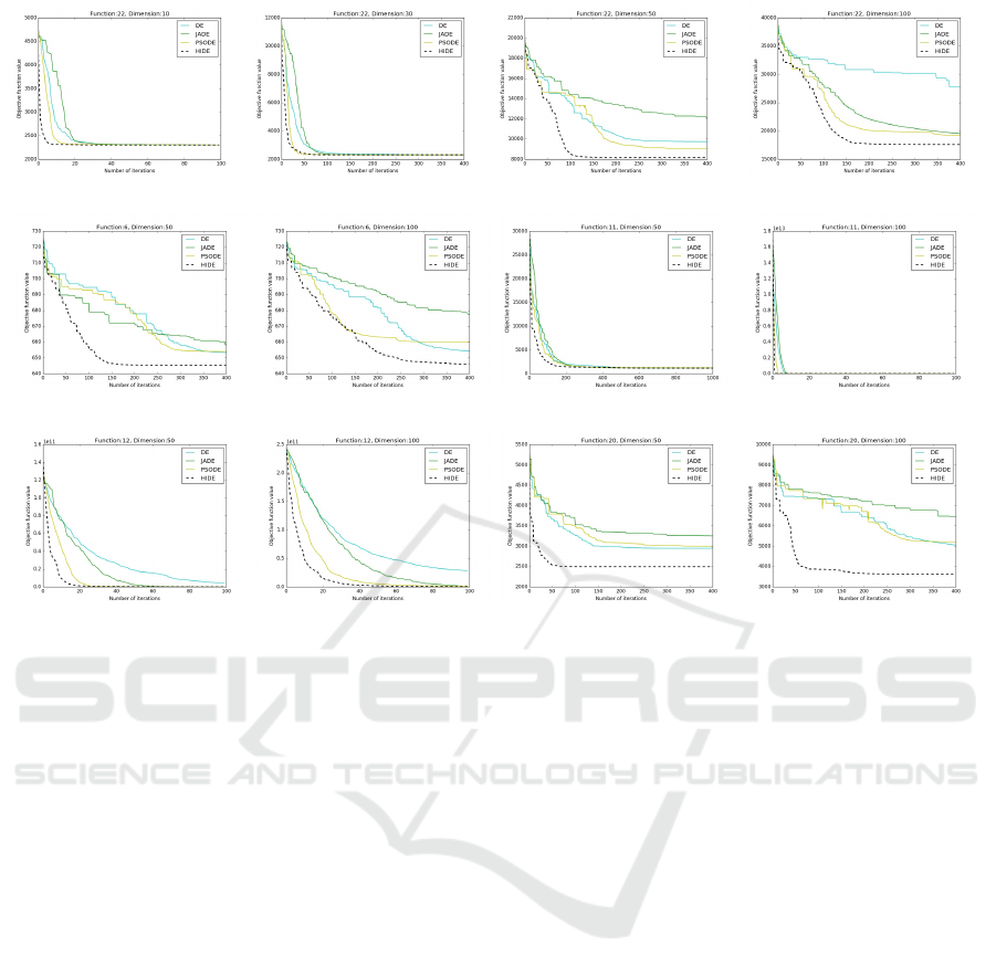
(a) (b) (c) (d)
(e) (f) (g) (h)
(i) (j) (k) (l)
Figure 4: Comparative convergence profiles for test functions from CEC 2017 Benchmark over D = 10,30,50,100.
rate.
The results for D = 50 and D = 100 (higher di-
mensions) have been summarized in tables 3 and 4.
On D = 50, HIDE depicted exceptional performance,
outperforming all other algorithms. It registered 17
wins in the best case and 18 wins in the mean case.
Classical DE shows no wins in any case in high di-
mensional settings owing to its slow convergence rate
and inability to attain global optimum thus highlight-
ing the usefulness of the modifications introduced in
the variants including HIDE. Similarly for D = 100,
HIDE again outperforms all other algorithms by an
appreciable margin. From a functional standpoint,
It would be worthwhile to highlight that HIDE out-
performed the other 3 compared algorithms on ma-
jority on the composite and hybrid functions, partic-
ularly on the higher dimensional settings. The effi-
ciency of HIDE can be attributed to the hierarchical
nature of crossover selection and concurrency in vec-
tor configurations at the higher hierarchy levels. The
tabular results reinforce the fact that HIDE outper-
forms JADE, PSODE and DE. On close analysis, it
can be witnessed that HIDE falls behind the other al-
gorithms on a small fraction of unimodal functions
such as f
5
, f
7
on lower dimensions due to fast con-
vergence during early stages of execution. However,
the performance of higher dimensions, particularly on
the more involved functions highlights utility for real
world problems.
The tabular results are complemented through the
graphical representations in Figure 4. For the sake of
clarity, representations of higher dimensional prob-
lems span more number of iterations than those for
lower dimensional settings. Analysis of the plots
clearly depicts that HIDE shows better convergence
rate as compared to other algorithms. As the analy-
sis transcends to higher dimensional settings, the pro-
posed approach outperforms the other algorithms on
majority of the objective functions with respect to
both convergence rate and optimality. the superiority
of our algorithm in higher dimensions (50 and 100)
is clearly evident from Figure 4 (c,d,g,h,k,l). Figure
4 (a,b,i,j) depict that for functions where HIDE and
the other variants may depict similar trends on lower
dimensions, HIDE eventually excels and surpasses
them in higher dimensions in most scenarios. Almost
all figures are representative of a faster convergence
rate for HIDE on higher dimensions. This remarkable
trait in HIDE enhances its utility for high dimensional
problems where fast convergence to global optimum
value is required, hence making it superior to the other
considered algorithms and several variants of the DE
algorithm.

5 CONCLUSION
Differential Evolution has been regarded as one of the
most successful optimization algorithms and over the
years, several variants have been proposed to enhance
its convergence rate and performance. In the present
work, we introduced a hierarchy influenced variant of
the classical DE algorithm and modeled the same on
the brain motor operation. The algorithm was char-
acterized by global leader, local leaders and an ef-
fector population. The global leader and distributed
local leaders interacted to facilitate gross motion via
a greedy exploration strategy. The local leaders and
their effectors interacted to control intricate motion
for smooth convergence. A hierarchical crossover pa-
rameter was introduced to characterize the hierarchi-
cal transition between the two interactions. The influ-
ence of the vector configurations at the higher levels
of hierarchy enabled the algorithm to avoid local min-
ima in most objective functions. The same is comple-
mented through our result observations wherein we
significantly outperform several popular algorithm on
complex multimodal functions in higher dimensional
settings. Our proposed approach has sought to es-
tablish a viable tradeoff between fast optimization,
robust convergence and low number of control pa-
rameters. The performance analysis of the algorithm
highlights the particular effectiveness of the proposed
approach on high dimensional hybrid and composite
functions. The observed results provide sufficient mo-
tivation to extend the scope of the work to complex
high dimensional real life problems including image
enhancement, traveling salesman problem and flexi-
ble job-shop scheduling.
REFERENCES
Awad, N., Ali, M., Liang, J., Qu, B., and Suganthan, P.
(2016). Problem definitions and evaluation criteria for
the cec 2017 special session and competition on sin-
gle objective real-parameter numerical optimization.
Technical Report,.
Brest, J., Greiner, S., Boskovic, B., Mernik, M., and Zumer,
V. (2006). Self-adapting control parameters in differ-
ential evolution: A comparative study on numerical
benchmark problems. IEEE transactions on evolu-
tionary computation, 10(6):646–657.
Das, S. and Suganthan, P. N. (2011). Differential evolution:
A survey of the state-of-the-art. Evolutionary Compu-
tation, IEEE Transactions on, 15(99):4–31.
Dorigo, M. and St
¨
utzle, T. (2010). Ant colony optimiza-
tion: overview and recent advances. In Handbook of
metaheuristics, pages 227–263. Springer.
Hunter, J. D. (2007). Matplotlib: A 2d graphics environ-
ment. Computing In Science & Engineering, 9(3):90–
95.
Kennedy, J. and Eberhart, R. (1995). Particle swarm op-
timization. In Neural Networks, 1995. Proceedings.,
IEEE International Conference on, volume 4, pages
1942–1948 vol.4.
Liu, H., Cai, Z., and Wang, Y. (2010). Hybridizing parti-
cle swarm optimization with differential evolution for
constrained numerical and engineering optimization.
Appl. Soft Comput., 10(2):629–640.
Mezura-Montes, E. n., Vel
´
azquez-Reyes, J., and
Coello Coello, C. A. (2006). A comparative
study of differential evolution variants for global
optimization. In Proceedings of the 8th Annual Con-
ference on Genetic and Evolutionary Computation,
GECCO ’06, pages 485–492, New York, NY, USA.
ACM.
Oliphant, T. E. (2007). Python for scientific computing.
Computing in Science & Engineering, 9(3):10–20.
Onwubolu, G. C. and Babu, B. (2013). New optimization
techniques in engineering, volume 141. Springer.
Passino, K. M. (2002). Biomimicry of bacterial foraging
for distributed optimization and control. IEEE control
systems, 22(3):52–67.
Passino, K. M. (2005). Biomimicry for optimization, con-
trol, and automation. Springer Science & Business
Media.
Poli, R., Kennedy, J., and Blackwell, T. (2007). Particle
swarm optimization – an overview.
Shaw, D. M., Kellam, A., and Mottram, R. (1982). Brain
sciences in psychiatry. In Shaw, D. M., Kellam, A.,
and Mottram, R., editors, Brain Sciences in Psychia-
try. Butterworth-Heinemann.
Storn, R. and Price, K. (1995). Differential evolution-a sim-
ple and efficient adaptive scheme for global optimiza-
tion over continuous spaces, volume 3. ICSI Berkeley.
Van Der Walt, S., Colbert, S. C., and Varoquaux, G. (2011).
The numpy array: a structure for efficient numerical
computation. Computing in Science & Engineering,
13(2):22–30.
Zhang, J. and Sanderson, A. C. (2009). Jade: adaptive
differential evolution with optional external archive.
IEEE Transactions on evolutionary computation,
13(5):945–958.