
An Interactive Virtual Simulator for Motion Analysis of
Underwater Gliders
Alan López-Segovia, Luis García-Valdovinos, Tomás Salgado-Jiménez, Isabel Andrade-Bustos,
Luciano Nava-Balanzar, José Luis Sánchez-Gaytán and Juan Pablo Orozco-Muñiz
Energy, CIDESI, Av. Playa Pie de la Cuesta 702, 76125, Queretaro, Queretaro, Mexico
Keywords: Virtual Reality, Underwater Gliders, Modelling and Control, Haptic Interfaces.
Abstract: Autonomous Underwater Gliders (AUG) have become a very useful and cheap tool to sample the ocean’s
environment compared with oceanographic ships to perform the same task. AUGs can glide along the ocean
up to a specific depth thanks to their aerodynamic shape, wings and rudders, and a buoyancy-driven system
composed of a bladder and an eccentric movable mass that modifies the net buoyancy and the pitch/roll
angles of the vehicle, respectively. One of the main concerns of glider’s pilots is to understand and/or
predict the behaviour of the glider when it is affected by ocean currents under the water. In this paper, an
interactive virtual simulator for motion analysis of underwater gliders is given. The simulator considers the
online solution of the full nonlinear hydrodynamics of a well-known glider. The virtual simulator is a tool
that will help technicians and pilots to increase their training process, to carry out performance analysis of
new control schemes and validation of new glider’s models before the physical construction.
1 INTRODUCTION
An Autonomous Underwater Glider (AUG) bases its
operation on its buoyancy change to move through
the ocean in saw tooth patterns, reaching a specific
depth target. The AUG missions can explore
thousands of kilometres in long time missions
(several months) because of its low power
consumption. It can have different kinds of sensors
to analyse several water columns in ocean’s
environment following a zigzag trajectory until a
specific depth is reached; this vehicle has become
more and more popular for oceanographic studies
due to its low cost in comparison to traditional
methods. However, the cost of a commercial AUG is
not negligible so a real glider mission is considered a
critical task, therefore, a glider’s pilot must have a
full knowledge of the physical glider behaviour
under different environmental conditions (e.g.
marine currents) and inherent mission conditions
(e.g. velocity changes due to glider attitude). This
paper addresses the design and development of an
interactive virtual simulator for the study of the
behaviour of an AUG. The aim of this interactive
virtual simulator is to make the learning process
faster and easier for pilots before a real mission
deployment, performance analysis of new control
schemes and validation of new glider’s models
before the physical construction.
An interactive virtual simulator is a system
where can be reproduced the behaviour of a physical
phenomenon in a computer created environment
under conditions nearly to reality, the user can
handle the phenomenon parameters while simulation
is running. Through a virtual simulator can be either
predicted or analysed the phenomenon behaviour
without a physical implementation, virtual simulator
results are nearly approximated to real phenomenon
behaviour results. An AUG’s virtual simulator
development implies three main tasks: i) validation
and analysis of a mathematical model able to
reproduce real glider behaviour, ii) validation and
analysis of a mathematical model able to reproduce
environmental conditions wherein the AUG will
interact with, and iii) design of a virtual environment
(scenario and AUG graphical design and
animations) to give a real visual sensation for users.
Graver and Leonard (Graver & Leonard, 2001),
using a Newtonian approach, proposed a
mathematical model which sat the foundations to
obtain and do a formal analysis of AUG dynamics,
until that moment, a lot of AUGs had been used in
several successful oceanographic missions but
López-Segovia, A., García-Valdovinos, L., Salgado-Jiménez, T., Andrade-Bustos, I., Nava-Balanzar, L., Sánchez-Gaytán, J. and Orozco-Muñiz, J.
An Interactive Virtual Simulator for Motion Analysis of Underwater Gliders.
DOI: 10.5220/0006476804810488
In Proceedings of the 14th International Conference on Informatics in Control, Automation and Robotics (ICINCO 2017) - Volume 2, pages 481-488
ISBN: Not Available
Copyright © 2017 by SCITEPRESS – Science and Technology Publications, Lda. All rights reserved
481

neither a precise physical behaviour nor
mathematical properties had been comprehended
yet. Later, several research groups around the world
were dedicated to discover and understand physical
properties of that mathematical model (Bender,
Steinberg, Friedman, & Williams, 2008) (Ali
Hussain, Arshad, & Mohd-Mokhtar, 2011)
(Upadhyay, Singh, & Idichandy, 2015),
programming and computing the differential
equations system using a specific numerical method;
by their own, in (Wang, Singh, & Yi, 2013) a
Lagrangian approach has been used in order to
compute a mathematical model of the Slocum
Glider, a commercial AUG model. On the other
hand, the mathematical model presented in (Zhang,
Yu, & Zhang, 2013) captures general behaviour of
an AUG whose pitch and roll angles are generated
by an eccentric movable mass. Hydrodynamic
parameters are an important part of AUG
mathematical model that describe interaction
between vehicle and surrounding fluid and they
depend of fluid characteristics as well as vehicle
geometry. The hydrodynamic study of an AUG for
obtaining hydrodynamics parameters is a complex
task; currently there are a lot of commercial
computer software which can compute high
precision hydrodynamic parameters for complex
structures, under numerous simulated scenarios.
Using this techniques, there are several papers, like
(Zhang, Yu, & Zhang, 2013) (Seo, Jo, & Choi,
2008) (Seo & Williams, 2010) (Singh,
Bhattacharyya, & Idichandy, 2014), that employ a
CFD (Computational Fluid Dynamics) software to
estimate the coefficients and hydrodynamic forces of
an AUG.
In the literature are reported a number of AUG
simulators, most of them use the 2D mathematical
model presented in (Graver & Leonard, 2001), very
few use 3D mathematical model and none of them a
mathematical model implemented on a virtual
environment. A simulator presented in
(Phoemsapthawee, Le Boulluec, Laurens, & Deniset,
2013) represents an AUG with six degrees of
freedom. The objective of this work was the
hydrodynamic study of a vehicle to improve glider
designs and evaluate the control strategy
performance. The mathematical model used in this
work is based in Newton-Euler equations and
considers that mass centre is moved with respect to a
coordinate system fixed to the vehicle. Other work
about virtual simulator is presented in (Woithe &
Kremer, 2010), in this work a virtual simulator for
Slocum glider is presented. It’s not clear if the 3D
hydrodynamic model is used. In (Asakawa, Watari,
Nakamura, Hyakudome, & Kojima, 2013),
Tsukuyomi glider movements are observed
numerically, the depth effect produced in AUG’s
(water density change, AUG buoyancy, etc.) is
incorporated in the numerical simulation. This work
does not include interactive animations.
The discussion in this paper will procced as
follows: In section II the mathematical model used
for AUG behaviour and ocean environmental
reproduction is presented. Then, in section III
simulation testing and validation of mathematical
model is discussed. The AUG interactive virtual
simulator implementation is described in section IV.
Finally, conclusions are exposed in Section V.
2 MATHEMATICAL MODEL OF
AN UNDERWATER GLIDER
The mathematical model of an AUG used in the
interactive virtual simulator is proposed in (Zhang,
Yu, & Zhang, 2013); a well-known commercial
AUG model is incorporated in the interactive virtual
simulator. The model takes into account a moveable
eccentric mass for inducing a θ (pitch) angle and ϕ
(roll) angle.
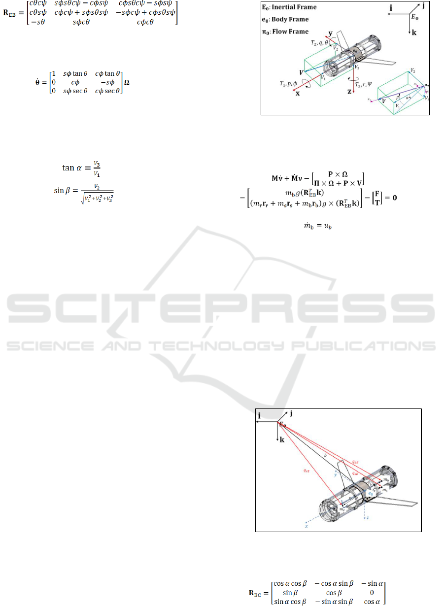
2.1 Kinematics Model
Figure 1 shows the coordinates frame used for the
AUG mathematical model calculation: Inertial
frame, body frame and flow frame, established to
describe the motion of the AUG. The body frame
origin
is established at the Buoyancy
Center (CB) of the AUG. The axis matches with
longitudinal axis of the AUG. The axis points
downward, forming 90° with axis. The axis lie
on the wings plane and is the result of the right hand
rule. The inertial frame is described by
,
where represents the frame axis and they are
unitary vectors. At the body frame, translational
velocity and angular velocity of the AUG are
defined as
and
,
respectively. At inertial frame, AUG position and
orientation are described by
and
, respectively. Rotation matrix
maps
of the body frame to the rate of change of at
inertial frame as follows:
(1)
Rotation matrix
is defined as:
ICINCO 2017 - 14th International Conference on Informatics in Control, Automation and Robotics
482
(2)
where
y .
The relationship between y
is given by:
(3)
Often is more useful and convenient to compute
and analyse at flow frame denoted by
in Figure 1. For flow frame definition,
first is necessary to define attack angle and
sideslip angle as follows:
(4)
(5)
The flow frame is defined with respect to body
frame as: First, the body frame is rotated by
angle around y axis, this yield that z axis is rotated to
a new position now called
axis. Later, the new
frame is rotated around
axis by angle. So,
both, axis is converted at
axis, and axis is
converted at
axis of flow frame.
2.2 Hydrodynamic Model
As mentioned above, the hydrodynamic model used
in the AUG’s interactive virtual simulator is
proposed in (Zhang, Yu, & Zhang, 2013), which can
reproduce the behaviour of any AUG’s.
Figure 2 shows mass distribution of an AUG:
static mass
, eccentric movable mass
, and net
buoyancy
which represents the difference
between total buoyancy () and AUG total mass
. The movable mass is modeled like
a half cylinder with eccentric offset
. Its mass
center is located at
along axis and it is rotated
by angle around axis. The vectors
and
denote mass center position of eccentric mass,
net buoyancy and static mass, respectively respect to
inertial frame. In turn, the vectors,
,
, and
express mass center position of eccentric mass, static
mass and net buoyancy respect to body frame,
respectively.
Figure 1: Coordinate frames.
The hydrodynamic equations that describe the AUG
behaviour are given by:
(6)
For more details refer to (Zhang, Yu, & Zhang,
2013).
2.3 Hydrodynamic Forces
In the flow frame, the hydrodynamic force
and hydrodynamic moment
are expressed as:
(7)
Figure 2: Mass distribution.
A rotation matrix
is defined as follows:
(8)
An Interactive Virtual Simulator for Motion Analysis of Underwater Gliders
483
maps the hydrodynamic force and
hydrodynamic moment from flow frame to body
frame as shown next:
(9)
2.4 Ocean Currents Model
In (Fossen, 2002) is described an ocean current
model widely accepted in underwater robotics.
Although the current model considers a laminar and
constant flow it is useful to analyse the
hydrodynamic behaviour of an AUG when this is
disrupted by a current with diverse directions and
intensities.
The ocean current model establishes that the
hydrodynamics can be expressed in terms of a
relative velocity as follows:
(10)
where
is the relative velocity between the
AUG velocity and the ocean current velocity
expressed in the body frame.
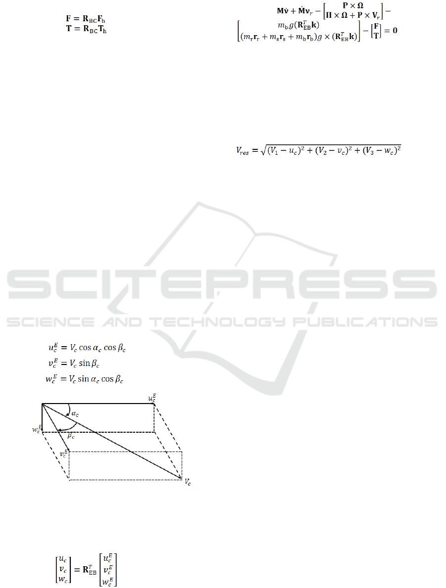
The ocean current components with respect to
inertial frame
can be related to
current intensity
defining two angles: attack angle
and sideslip angle
, which describe the
orientation respect to axis and axis, respectively,
as is shown in Figure 3.
The average ocean current velocity in terms of
attack angle and sideslip angle, expressed with
respect to the inertial frame is:
(11)
Figure 3: Flow frame.
To express the ocean current components from
inertial frame to body frame is necessary to use the
matrix
as follows:
(12)
The hydrodynamic model equations including
the ocean current effects now are described as:
(13)
where
. Now the mass, Coriolis-
centripetal and hydrodynamic force and moment
terms are only functions of acceleration and relative
velocity. For the hydrodynamic force and moment
described in (Graver J. , Thesis: Underwater Gliders:
Dynamics, control and design., 2005), the resultant
velocity in equation (6) is substituted by the next
resultant relative velocity:
(14)
3 MODEL VALIDATION
Once we have raised and analysed the AUG
hydrodynamic model, a validation of this becomes
necessary for its implementation in the AUG
interactive virtual simulator. The model validation is
made through a numerical simulation using the
mathematical software MATLAB/Simulink.
In a numerical simulation the results are shown
numerically through graphs for easy interpretation
and analysis. The variable values used for validation
model simulation are presented in Table I and Table
II.
Normally, an AUG does hundreds of cycles
during its mission, in one cycle the AUG sinks from
the ocean surface until a specific depth, then the
AUG rises from specific depth to ocean surface
again, that is one cycle end. For the model validation
the parameters for one cycle is summarized in Table
III and Table IV.
The eccentric mass is held at γ=0 (ϕ=0) at all time
to avoid inducing a turn in the AUG. Notice that the
Slocum glider induces a turn in the yaw angle by
means of an actuated rudder. Depending on the AUG
position the movable mass is moved to produce the
desired pitch angle .
ICINCO 2017 - 14th International Conference on Informatics in Control, Automation and Robotics
484
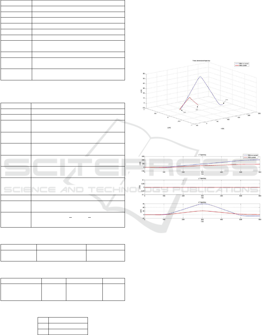
Table 1: Physical parameters of Slocum glider (Bardolet,
2012) (Teledyne Webb Research, 2012).
Variable
Value
@
(water mass displaced by the
vehicle @
)
(rudder area)
Table 2: Hydrodinamic parameters of slocum glider
(BARDOLET, 2012).
Variable
Value
,
(rudder angle of rotation)
Table 3: Sinking trajectory conditions.
0 – 50 s
50 – 150 s
150 – 250 s
Table 4: Rising trajectory conditions.
250 – 350 s
350 – 450 s
450 – 550 s
550 – 600 s
Table 5: Ocean current parameters.
0.12 m/s
180°
0°
Figures 4 and 5 depict the behaviour of the Slocum
glider with and without ocean currents. Evidently,
when ocean current is present the glider is restricted
to move freely.
The hydrodynamic model raised shows a
coherent behaviour with reality and reported data in
literature. Numerically, as is shown in Figure 4 to 5,
it presents good stability which is reflected with
moderate transition and low frequency signals. Thus,
the hydrodynamic model with and without current
effects is validated and available for its incorporation
in the AUG interactive virtual simulator.
Figure 4: Glider behavior during a cycle, wih and without
ocean current.
Figure 5: Trajectories followed by the glider with and
without ocean current.
Next, the main contribution of the paper is given.
4 GLIDER SIMULATOR
IMPLEMENTATION
The AUG interactive virtual simulator was created by
using a set of software tools such as Unity 3D,
Blender, Visual C++ and Matlab/Simulink. Figure 6
shows the combination of this Software tools.
An Interactive Virtual Simulator for Motion Analysis of Underwater Gliders
485
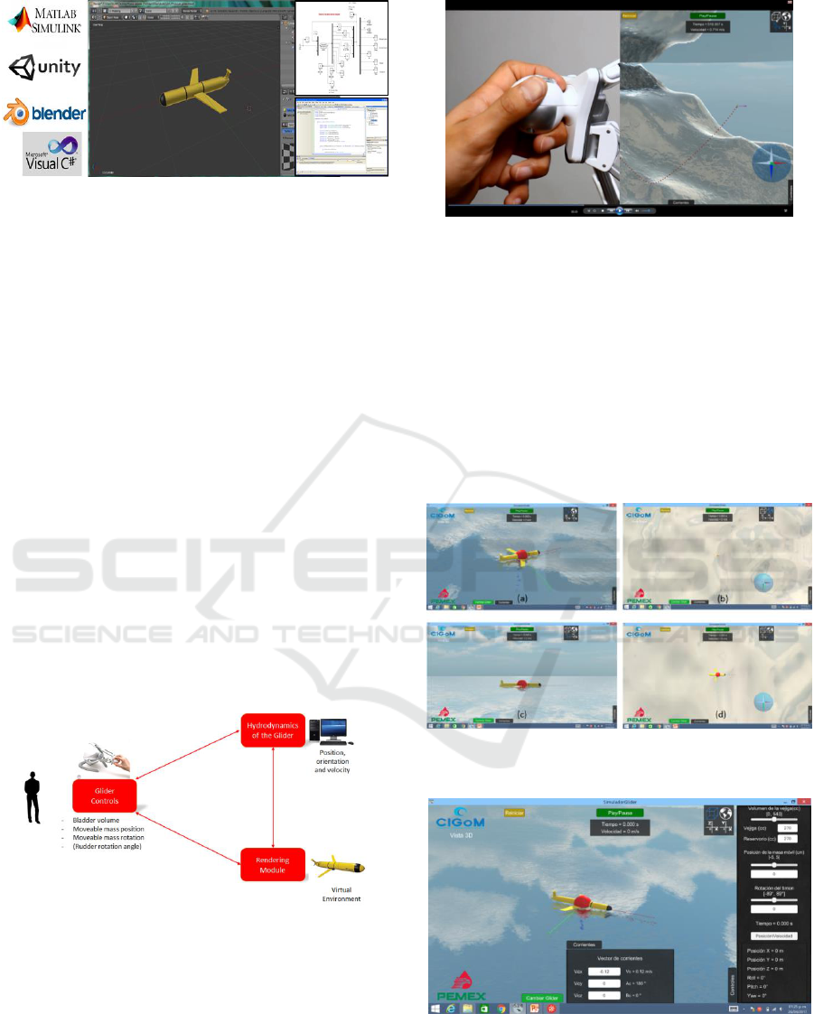
Figure 6: Software tools used for the development of the
interactive virtual simulator.
Unity 3D is one of the most popular and powerful
game engines used for the development of virtual
environments. Unity works as a platform that offers a
variety of tools to develop realistic scenarios along
with the capability to interface with scripts performed
in Visual C# and to import CAD models from
Blender.
The mathematical model along with the
parameters of each glider was added to the virtual
simulator using script files under C# language, inside
this script files was programmed the Heun numerical
integrator for the model resolution.
In Figure 7 a block diagram of the interactive
virtual simulator is displayed. The virtual simulator is
formed by a high performance PC and a haptic
interface (Falcon) which can be operated by the user
for controlling the AUG control. As shown above, in
the high performance computer the hydrodynamic
model is programmed which is solved online by the
Heun integrator. The model solution is processed by
the render module to recreate visually the AUG
motion in the virtual environment.
Figure 7: Block diagram of the interactive virtual
simulator.
The interactive virtual simulator allows the users
(pilots) to analyse the AUG motion in the 3D virtual
environment by manipulating the control variables
(bladder volume, moveable mass position and
moveable mass rotation), as shown in Figure 8.
Figure 8: The pilot can modify online the main variables
of the selected glider by means of a haptic interface, a
mouse or the keyboard.
The main screen displays three different types of
information and two types of controllable variables.
The types of information are: 3D visualization,
graphic visualization of variable values and
numerical visualization of AUG state variables. The
types of controllable variables are: AUG control
variables and ocean current velocity. Figure 9 and
Figure 10 depicts, respectively, the 4 different views
and the control variables and ocean current panels.
Figure 9: (a) Isometric view, (b) Superior view (Gulf of
Mexico map), (c) plane view, (d) plane view.
Figure 10: Control variables and ocean current control
panels.
Finally, it includes a button which allows choosing
between the AUG 3D models: Seaglider, Slocum,
ICINCO 2017 - 14th International Conference on Informatics in Control, Automation and Robotics
486
Seawing and soon the CIDESI’s glider. Any other
commercial or academic glider can be added to the
simulator provided the whole parameters are
available. When the AUG 3D model is chosen the
corresponding hydrodynamic model and parameters
are chosen too. Once a simulation is running is not
possible to change the AUG model until the button
“Restart” is pushed.
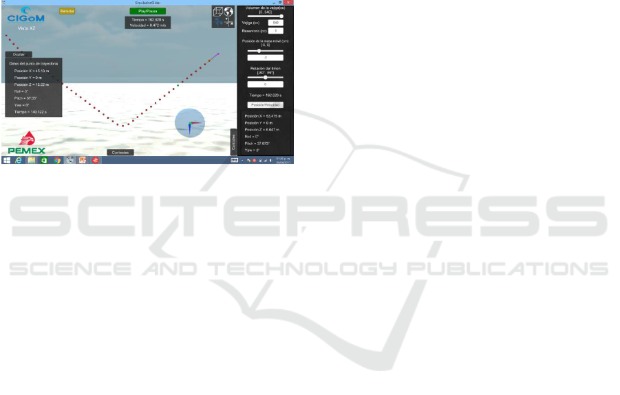
Each control panel is fitted with a button to
expand or collapse the information. While the
simulation is running the AUG creates navigation
marks, which stores historical data about AUG
trajectory, as can be seen in Figure 11.
Figure 11: Equidistant navigation marks (red balls) draw
the glider trajectory. A green ball is a particular point
selected by the pilot to know the glider’s state in the
inertial frame.
5 CONCLUSIONS
In this paper, preliminary results of an interactive
virtual simulator are presented. The simulator solves
online the full nonlinear hydrodynamics of
underwater gliders and the solution is fed to the
rendering module (virtual environment) to display
the motion in a realistic 3D scenario in order to
analyze the behavior. The simulator is provided with
different tools to analyze the motion and the
generated information. At this moment, the virtual
simulator is interactive; it means that the pilot can
modify online the three main control variables of an
underwater glider: volume of the bladder, position of
the moveable mass and the rotation angle of the
eccentric mass. In the case of the Slocum glider, an
actuated rudder has been considered into the
hydrodynamics instead of the eccentric mass.
Additionally, the simulator has a panel to arbitrarily
set the intensity and direction of the ocean current.
The simulator represents a useful tool for the
Oceanographic Monitoring Group with Gliders
(GMOG) pilots.
Future work is to implement the functionality of
“automatic mode” and add the map of the Gulf of
Mexico wherein the pilot will be able to indicate on
it the starting point and the subsequent way points
that the glider has to reach, with or without currents.
Not only the virtual environment and the graphic
user interface have to be modified but also it is
necessary to choose the correct control law.
ACKNOWLEDGMENT
This study is part of the project number 201441
“Implementation of oceanographic observation
networks (physical, geochemical, ecological) for
generating scenarios of possible contingencies related
to the exploration and production of hydrocarbons in
the deepwater Gulf of Mexico”, granted by SENER-
CONACyT Hydrocarbons Sectorial Fund.
REFERENCES
Ali Hussain, N. A., Arshad, M. R., & Mohd-Mokhtar, R.
(2011). Underwater glider modelling and analysis for
net buoyancy, depth and pitch angle control. Ocean
Engineering, 38(16), 1782 - 1791.
Asakawa, K., Watari, K., Nakamura, M., Hyakudome, T.,
& Kojima, J. (2013). Motion Simulator for an
Underwater Glider for Long-term Virtual Mooring
Including Real Devices in Loop. IEE/MTS Oceans.
Bardolet, A. (2012). Contributions to Guidance and
Control of Underwater Gliders. Master Thesis,
University of Southern Denmark.
Bender, A., Steinberg, D., Friedman, A., & Williams, S.
(2008). Analysis of an autonomous underwater glider.
Australasian Conferencie on Robotics and
Automation. Canberra, Australia.
Fossen, T. (2002). Marine Control Systems Guidance,
Navigation, and Control of Ships, rigs and
Underwater Vehicles. Marine Cybernetics.
Graver, J. (2005). Thesis: Underwater Gliders: Dynamics,
control and design. Mechanical and Aerospace
Engineering.
Graver, J. G., & Leonard, N. E. (2001). Underwater Glider
Dynamics and Control. 12th International Symposium
on Unmanned Untethered Submersible Technology.
Durham.
Graver, J., Bachmayer, R., & Leonard, N. (2003).
Underwater Glider Model Parameter Identi_cation.
Proceedings 13th International Symposium on
Unmanned Untethered Submersible Technology
(UUST).
Graver, J., Liu, J., Woolsey, C., & Leonard, N. (1998).
Design and Analysis of an Underwater Vehicle for
Controlled Gliding. Princeton University. Conference
on Information Sciences and Systems (CISS).
An Interactive Virtual Simulator for Motion Analysis of Underwater Gliders
487

Phoemsapthawee, S., Le Boulluec, M., Laurens, J., &
Deniset, F. (2013). A Potential Flow Based Flight
Simulator for an Underwater Glider. Journal of
Marine Science and Application, 12, 112-121.
Seo, D., & Williams, C. (2010). CFD Predictions of Drag
Force for a Slocum Ocean Glider. National Research
Council Canada.
Seo, D., Jo, G., & Choi, H. (2008). Pitching Control
Simulations of an Underwater Glider Using CFD
Analysis. OCEANS. Kobe.
Singh, Y., Bhattacharyya, S., & Idichandy, V. (2014).
CFD Approach to Steady State Analysis of an
Underwater Glider. IEEE/MTS Oceans. St. Johns,
Canada.
Teledyne Webb Research. (2012). Slocum G2 Glider
Maintenance Manual. East Falmouth, MA: Teledyne
Webb Research.
Upadhyay, V. K., Singh, Y., & Idichandy, V. (2015).
Modelling and Control of an Underwater Laboratory
Glider. Underwater Technology (UT), 2015 IEEE.
Wang, P., Singh, P. K., & Yi, J. (2013). Dynamic Model-
Aided Localization of Underwater Autonomous
Gliders. IEEE International Conference on Robotics
and Automation (ICRA). Karlsruhe, Germany.
Woithe, H. C., & Kremer, U. (2010). An Interactive
Slocum Glider Flight Simulator. IEE/MTS Oceans.
Zhang, S., Yu, J., & Zhang, F. (2013). Spiraling motion of
underwater gliders: Modeling, analysis, and
experimental results. Ocean Engineering, 60, 1-13.
ICINCO 2017 - 14th International Conference on Informatics in Control, Automation and Robotics
488
