
Tracking Solutions for Mobile Robots: Evaluating Positional Tracking
using Dual-axis Rotating Laser Sweeps
Sebastian P. Kleinschmidt, Christian S. Wieghardt and Bernardo Wagner
Real Time Systems Group, Institute of Systems Engineering, Leibniz Universit
¨
at Hannover,
Appelstraße 9A, 30167 Hannover, Germany
Keywords:
Tracking Technologies, Marker Tracking, Dual-axis Rotating Laser Sweeps.
Abstract:
This paper provides a comprehensive introduction into state of the art marker-based tracking methods. There-
fore, optical, magnetic, acoustic and inertial tracking are described and evaluated. All presented approaches
are compared regarding accuracy, resolution, tracking volume, measurement rate and outdoor and indoor suit-
ability. Additionally, typical technical limitations are mentioned for each system according to their functional
principle.
As a technology with increasing potential for mobile robotics, we evaluate the achievable accuracy for pose
tracking using dual-axis rotating laser sweeps as used in modern tracking systems for virtual reality applica-
tions.
1 INTRODUCTION
In many applications, the pose of an object, a robot or
an instrument needs to be determined as accurate as
possible. Examples of such applications are medical
engineering, augmented reality and mobile robotics.
A detailed overview of tracking systems in medical
applications is presented in (Birkfellner et al., 2008).
In general, there are two basic solutions for determin-
ing and tracking the pose of an object: Marker- and
non marker-based systems. Due to higher accuracy,
marker-based tracking systems have been established
as the standard solution for pose measurements which
can be used as ground truth for many research areas
to evaluate the performance of developed algorithms.
This paper gives a general overview of tracking sys-
tems, which can be used in robotic applications.
This paper is organized as follows: The first sec-
tion introduces evaluation criteria which can be used
to compare state of the art marker-based tracking sys-
tems. Then, the functional principles of different sys-
tems as optical, magnetic, acoustic and inertial sys-
tems are described. Subsequently, a comparison of
the approaches is presented. The results are given in
a comprehensive table. The paper ends with an eval-
uation of a tracking system based on dual-axis rotat-
ing laser sweeps. Experiments are performed using
a trackable handheld device as well as a Pioneer 2
robot.
2 EVALUATION CRITERIA
All tracking systems considered in this paper will be
evaluated based on the criteria presented in this sec-
tion. If possible, we will quantify the results by speci-
fications of commercial tracking systems or scientific
publications.
Accuracy: According to ISO 5725, accuracy consists
of trueness and precision. Trueness describes how
close the mean of a set of measurements results to
the true value, whereas precision describes the degree
of scattering of the set of measurements. In tracking
applications, trueness and precision may vary if the
observed object is static or moving. Based on this
fact, to evaluate tracking systems, it is necessary to
differentiate between static accuracy and dynamic ac-
curacy:
Static Accuracy: Static accuracy describes the accu-
racy which can be achieved for a non-moving object.
Dynamic Accuracy: Analogue to the static accuracy,
the dynamic accuracy is used for moving objects.
Resolution: The resolution of a tracking system is the
smallest yet to distinguish difference in position and
orientation which can be measured by the system.
Tracking Volume: The space in which a tracking
system tracks objects, is called tracking volume. This
tracking volume is described by geometric primitives,
for which tracking is provided within defined accu-
racy boundaries. The achievable accuracy may vary
within this volume.
Kleinschmidt, S., Wieghardt, C. and Wagner, B.
Tracking Solutions for Mobile Robots: Evaluating Positional Tracking using Dual-axis Rotating Laser Sweeps.
DOI: 10.5220/0006473201550164
In Proceedings of the 14th International Conference on Informatics in Control, Automation and Robotics (ICINCO 2017) - Volume 1, pages 155-164
ISBN: 978-989-758-263-9
Copyright © 2017 by SCITEPRESS – Science and Technology Publications, Lda. All rights reserved
155

Measurement Rate: The measurement rate defines
how many pose updates can be generated in a defined
time period.
Indoor and Outdoor Suitability: Based on the func-
tion principle of the used tracking system, the system
can be affected by external factors such as direct sun-
light. Therefore, not all systems are equally suited for
outdoor applications and need a controlled environ-
ment.
3 OPTICAL SYSTEMS
Traditional optical tracking systems consist of one or
more cameras which are placed rigidly in the envi-
ronment. The tracking volume is defined by the re-
sulting overlapping field of view (fov) of the cameras.
To track the position of a marker, the marker has to
be visible in at least two cameras with a direct line-
of-sight. Except are tracking approaches using pre-
defined pattern such as fiducial marker which can be
tracked by a single camera (see Section 3.1).
The accuracy of an optical system is mainly deter-
mined by the resolution of the used cameras, the fov
given by the used lenses, the distance to the measured
markers and the distance between the cameras in case
of using multiple cameras.
The measurement rate is limited by the framerate
of the cameras and can be further limited by the pro-
cessing time which is needed to identify the maker or
pattern structure. In case of using multiple cameras,
the cameras need to be time synchronized. To sim-
plify the identification of the marker position in the
camera images, typical markers are coated with a re-
flective material which is illuminated by light sources
arranged around the camera lenses (LEDs in most ap-
plications). To further facilitate the marker identifi-
cation and prevent the influence of ambient light, the
light sources often emit light in the infrared spectrum
(e.g. 850 nm) which is filtered by an optical band-pass
filter in front of the camera lenses.
Besides passive concepts, there are also ac-
tive markers which are mostly battery powered and
equipped with a light source (e.g. LEDs) inside the
marker enclosure. There are also optical tracking sys-
tems which work without cameras such as laser track-
ing systems. In this kind of systems, the cameras are
replaced by rotating planes of coherent lasers light
which are detected using an array of photosensors.
Laser based systems are described at the end of this
section.
(a) Concentric Cir-
cles
(b) Intersense (c) ARToolkit
(d) ARTag. (e) RUNE-43. (f) RUNE-129.
Figure 1: Examples of common fiducial markers (Bergam-
asco et al., 2011).
3.1 Single View Systems
The most basic setup for an optical tracking system is
a single camera setup. Because tracking is not pos-
sible using triangulation with a spherical marker be-
ing visible in only one camera, it is necessary to use
marker with predefined pattern as fiducial marker.
Besides typical spherical markers, it is common
for simple applications to use fiducial markers as
augmented reality tags or other predefined patterns.
These markers are placed in the camera’s fov as a
point of reference. The resulting transformation be-
tween the pose of the marker and the camera can then
be computed using conventional algorithms that solve
the perspective-n-point problem. Typical applications
for the usage of fiducial marker are augmented real-
ity applications in mobile applications where virtual
models are rendered into the camera image based on
the computed transformation between the camera and
the AR-Tag. Examples of fiducial markers are shown
in Figure 1.
The accuracy of tracking a Metaio marker using
a single camera has been evaluated in (Pentenrieder
et al., 2006) using a simulated ground truth. The
accuracy of Metaio marker detected by a simulated
640 ×480 (15 fps) camera has been evaluated from
different distances and from different rotation angles.
The accuracy of optical tracking with an AR-
ToolKit fiducial marker has been evaluated in (Abawi
et al., 2004) using a camera with a resolution of
640 ×480 (15 fps). The systematic error was given
by 2 cm in a distance of 20 cm and increases at higher
distances.
The tracking volume for fiducial maker tracking is
limited by the fov and the resolution of the used cam-
era. The setup for a single camera tracking is sim-
ICINCO 2017 - 14th International Conference on Informatics in Control, Automation and Robotics
156
P(x,y,z)
P
1
(x,y)
P
2
(x,y)
b
x
z
f
c
1
c
2
y
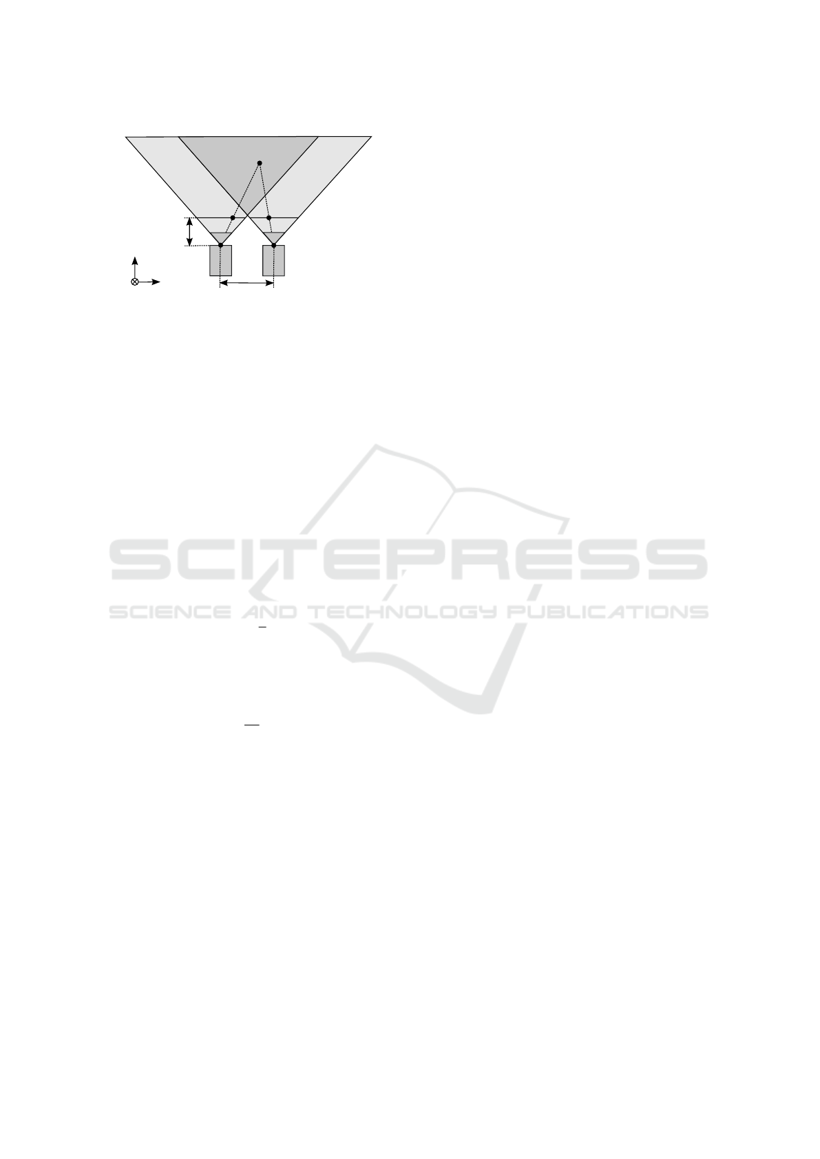
Figure 2: The basic setup of a stereo tracking system. The
resulting tracking volume is marked dark gray.
ple because no time synchronization between differ-
ent cameras needs to be performed and there is only
an intrinsic calibration of one camera necessary. It
is possible to determine the 6-dof transformation of a
marker inside the camera’s fov.
3.2 Stereo View Systems
Stereo-based tracking systems consist of two cameras
which are placed in a rigid geometric relation to each
other, and therefore have to be extrinsically and in-
trinsically calibrated. Figure 2 shows the basic setup
of a stereo tracking system.
To triangulate the distance of a marker, both cam-
eras need to be time synchronized. The depth of a
marker Z given its disparity d can then be computed
as follows (Szeliski, 2010):
Z = f
b
d
. (1)
The theoretical depth resolution of a stereo camera
system has been evaluated in (Mikko Kyt, 2011) and
can be computed for the overlapping fov of both cam-
eras:
dZ =
Z
2
f b
d p
x
. (2)
The theoretical depth resolution of a stereo system dZ
depends on the focal length f , the baseline between
both cameras b and the disparity accuracy d p
x
. For a
constant image resolution, d p
x
increases with a grow-
ing fov wherefore the depth resolution impair.
While a small baseline b minimizes the regions
of the image, where partial occlusions can occur, the
depth uncertainty grows, because of a small triangu-
lation angle. In contrast, a large baseline b increases
the chance of an object only to be visible in one image
but also increases the depth accuracy. Commercial
stereo systems reach an accuracy of about 0.35 mm
in a tracking volume up to approx. 1.6 m
3
(Andrew
D. Wiles and Frantz, 2004).
Because the tracking volume is limited to the over-
lapping area of both cameras, the resulting tracking
volume is smaller than the tracking volume which
could be achieved with a single view system.
3.3 Multi-view Systems
In multi-view systems (also known as multi-view
stereo), the marker must be visible in at least two cam-
eras at the same time to perform triangulation. While
depth estimation is already possible with two cam-
eras, matching more images can be used to increase
the tracking volume and make the system more ro-
bust against occlusions. One major factor for gaining
high accuracy is to track objects with two cameras at
perpendicular line of sights and small distances to the
objects. Therefore, stereo view systems have a limited
tracking volume with high accuracy. Whereas multi-
view systems can easily deploy additional cameras in
the tracking volume to increase such conditions, not
for a significant higher accuracy, but for a larger high
accurate tracking volume.
3.4 Laser Systems
Laser tracking systems are optical systems which
work without the usage of cameras (in contrast to the
optical approaches presented before). Instead of us-
ing passive or active markers which are detected in a
camera image, the markers are replaced with an array
of photosensors in a known geometric arrangement
which are illuminated by two or more rotating planes
of coherent lasers light. Therefore, the concept is also
named dual-axis rotating laser sweeps, because every
emitter is rotating two different laser planes. The po-
sition of the sensor array relative to the emitter is com-
puted by sampling the position of the laser plane and
the signal from the photosensors (Birkfellner et al.,
2008).
While the outdoor suitability of laser-based track-
ing systems is determined by the wavelength and the
power of the emitting light source, the possible track-
ing volume is mainly determined by the emitting an-
gles of the laser planes which are rotated. Besides,
the maximal distance between tracked device and the
emitting base station is limited by the power of the
emitting light source. The static resolution, which is
achieved by a commercial laser tracking system, is
given with 0.1 mm at a distance of 1 m (laserBird 2
by Ascension Technology Corporation working at a
measurement rate of 250 Hz (Ascension Technology
Corporation, 2000).
While laser tracking systems are not often used in
medical applications (Birkfellner et al., 2008), they
are interesting for head tracking in virtual reality ap-
plications based on the possible high frame rate and
Tracking Solutions for Mobile Robots: Evaluating Positional Tracking using Dual-axis Rotating Laser Sweeps
157
3-Axis
Magnetic
Source
Field Coupling
Position and Orientation
Measurements
Driving
Circuits
Computer
Amplifying
Circuits
3-Axis
Magnetic
Sensor
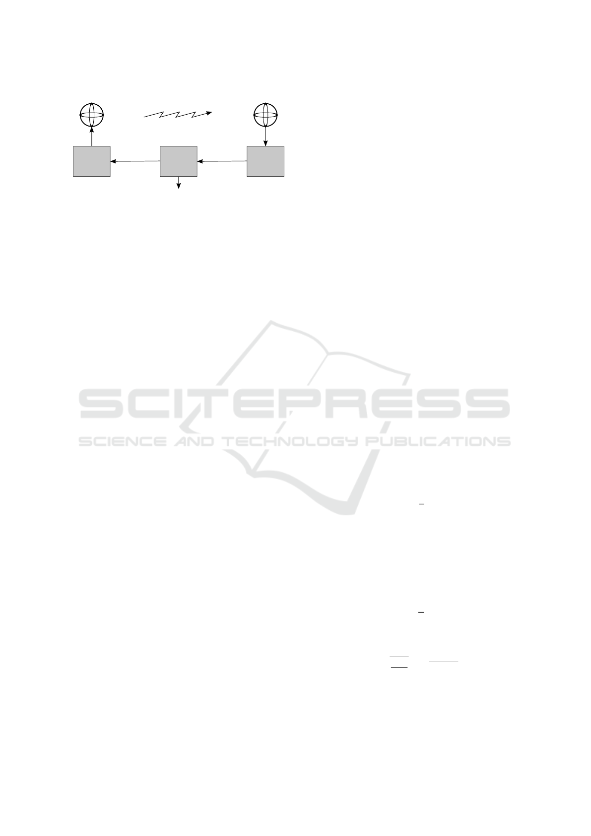
Figure 3: Magnetic coupling (based on figure presented in
(Raab et al., 1979)).
low latency (which is necessary to avoid simulator
sickness). Laser-based systems have become a highly
available consumer product due to the usage in the
HTC Vive virtual reality headset. Whereas the HTC
Vive includes two controllers in addition to the head-
set, the system can be extended by stand alone track-
able devices called HTC Trackers, which provide 6-
dof tracking information. When this paper was writ-
ten, the HTC Tracker were not yet available for pur-
chase.
4 MAGNETIC SYSTEMS
Magnetic tracking systems consist of multiple
magnetic emitters and one or more sensors whose
position and orientation are tracked. In most systems,
the source has three orthogonal coils which generate
individual perpendicular magnetic fields and induce
currents in the three orthogonal coils of the sensor
(Raab et al., 1979). The amplitudes of the nine
measured currents result in the position of the sensor,
a comparison delivers the orientation. Small changes
of the source position and orientation are determined
and the previous measurements are updated. There
are also alternative methods that use just two coils
(Paperno et al., 2001) or a magnet (Hu et al., 2007) as
a source. The basic structure of a magnetic tracking
system is presented in Figure 3.
There are altering current (AC) and direct current
(DC) based magnetic tracking systems. In AC sys-
tems, a signal sequence on a high carrier frequency
wave is transmitted. The signal induces eddy cur-
rents in conductive materials nearby and therefore
also small local electromagnetic fields which inter-
fere with the measurements. DC-based magnetic sys-
tems generate pulsed constant magnetic fields. That
prevents disturbances by conductive materials since
eddy currents vanish fast enough. Whereas, constant
magnetic fields such as the Earth’s fields or caused by
ferromagnetic materials can vary the measurements.
Hence, the trueness of the magnetic tracking strongly
depends on its environment.
Since the induced field penetrates all sorts of ma-
terials, the tracking does not depend on a direct line-
of-sight and are therefore not affected by occlusions.
The method is also independent of lightning condi-
tion, thus is not restricted to indoor utilization.
Commercial magnetic tracking systems achieve
a static precision of 0.76 mm RMS and 0.15
◦
resp.
RMS at a distance of 762 mm (FASTRACK by Pol-
hemus Inc. (Polhemus, 2017a)). The system has a
measurement rate of 120 Hz and a latency of 4 ms.
The resolution is given by 0.0058 mm and 0.0026
◦
at a distance of 304.8 mm and rapidly decreases with
the displacement between source and sensor. At a dis-
tance of 3048 mm only a resolution of 40.64 mm and
2.96
◦
resp. can be achieved. The range is limited
to 10 feet but can be extended to 30 feet. There are
also wireless magnetic tracking systems available e.g.
(PATRIOT WIRELESS by Polhemus Inc. (Polhemus,
2017b)). They support a higher range, but suffer a
loss in accuracy.
5 ACOUSTIC SYSTEMS
Acoustic tracking systems use the duration of ultra-
sonic waves to determine the position of the marker.
For this purpose, the object is equipped with an ul-
trasonic transmitter as a marker while receivers are
placed statically on defined locations in the environ-
ment. The position of a transmitter can then be deter-
mined by triangulating the time of flight of the ultra-
sonic waves.
Based on the limited propagation speed of ultra-
sonic waves in air (c≈ 343
m
s
at 20
◦
C) the maximal
update rate f is limited according to Equation 3. Be-
cause the propagation speed depends on the environ-
mental conditions like temperature and pressure, the
measurement of the time of flight needs to be fused
with other sensors measuring these influencing fac-
tors to determine the correct distance. Furthermore,
the time of flight can be affected by obstacles between
the transmitter and the receiver.
f =
c
d
(3)
The propagation speed c for different gases can be
computed according to Equation 4.
c =
r
κ ·p
ρ
=
√
κ ·R ·T , (4)
with the adiabatic exponent κ, the pressure of the gas
p, and the density of the gas ρ and R being the general
gas constant.
ICINCO 2017 - 14th International Conference on Informatics in Control, Automation and Robotics
158

The work presented in (Priyantha et al., 2000) de-
scribes a system called Cricked whose setup is in-
verse to the description above: The emitter are placed
static in an indoor environment and the receivers are
kept mobile on a robot for position tracking. The sys-
tem achieves a location granularity of 4x4 square feet
(Priyantha et al., 2000).
(Ward et al., 1997) presents a system called Active
Bats which operates in a volume of 1100 m
3
using 256
ultrasonic receivers. The trueness of Active Bats is
given with 9 cm for 95 % of the measurements with an
update rate of 25 Hz (Hightower and Borriello, 2001)
(Ward et al., 1997).
Compared to other tracking solutions, the price of
an ultrasonic based tracking system is low (the price
of each device used for the Cricked system costs less
than 10 USD (Priyantha et al., 2000)). The propa-
gation speed limits the update rate of systems based
on ultrasonic time of flight measurements. Ultrasonic
based systems are inaccurate compared to other track-
ing systems, can be disturbed by reflecting ultrasonic
signals and are therefore not often used in state of the
art applications.
6 INERTIAL SYSTEMS
Inertial navigation systems (INSs) use inertial mea-
surement units (IMUs) as markers with no external
tracking system to track the position of an object start-
ing from a known initial position and orientation with
a known initial velocity. These initial information are
then combined with the output of the IMU to compute
the position, velocity and attitude of the object (No-
vAtel, 2014). An IMU typically consists of a three-
axis gyroscope and a three-axis accelerometer. Fur-
thermore, there are also hybrid IMUs (magnetic, an-
gular rate and gravity - MARG) available which in-
clude an additional three-axis magnetometer. INSs
are divided into two different categories (Noriega-
Manez, 2007) (Woodman, 2007):
• Stable Platform Systems (also known as Gimbal-
Mounted or Mechanized Systems)
• Strap-Down Systems
Stable Platform Systems are mounted on a platform
using gimbals to isolate the IMU from any external
rotational motion (Woodman, 2007). The gyroscopes
of the IMU are then used to measure occurring rota-
tions to keep the platform’s rotation static regarding
a global frame of reference using servo motors. The
orientation of the system can then be determined
by reading the servo encoders. The position of
the system is computed by double integrating the
Orientation
Servo
Feedback
Initial Position
Initial Velocity
Global
Accel
Velocity
∫
∫
Accelerometer
signals
Correct for
gravity
Position
Figure 4: Stable platform inertial navigation algorithm
(based on figure presented in (Woodman, 2007)).
Orientation
Rate-gyroscope
signal
Accelerometer
signal
Position
Initial Position
Initial Velocity
Project
accelerations
onto global
axes
Correct for
gravity
Global
Accel
Velocity
∫
∫
∫
Initial
Orientation
Figure 5: Strapdown inertial navigation algorithm (based on
figure presented in (Woodman, 2007)).
acceleration which has to be corrected regarding
gravity before integration. The basic structure of a
stable platform inertial navigation algorithm is shown
in Figure 4.
Strap-Down Systems are mounted directly onto the
object with no additional mechanic structures and are
therefore smaller than stable platform systems. In
contrast to stable platform systems, strap-down sys-
tems can be rotated regarding the global frame and the
accelerometer needs to be transformed into the global
frame to correct the gravity. The position of the sys-
tem can then be computed by double integrating the
accelerometer signal (see Figure 5).
Signals from an IMU can typically be processed at
a high measurement rate (e.g. 200 Hz) (NovAtel,
2014). Because the signals are measured directly
at the object, there is no line-of-sight between the
marker and an external device necessary.
If the bias error of the accelerometer is not
removed, the error will be integrated twice as part
of the mechanization process which will lead to a
quadratic error in position computation (NovAtel,
2014). The same applies for the double integration of
measurement noise and an error-prone compensation
of gravity. Because the integration of the accelerom-
eter signals is error-prone, the resulting position
is strongly affected by drift. The average error in
position for a Xsens Mtx IMU was given with 150 m
after 60 s of operation (Woodman, 2007). For drift
reduction, the IMU signal often gets merged with
additional sensor signals as an absolute positioning
system (e.g. GPS for outdoor applications or optical
systems for indoor applications, see Section 3).
A full introduction to inertial navigation systems
(INSs) with a trial on error sources can be found in
(Woodman, 2007) (NovAtel, 2014).
Tracking Solutions for Mobile Robots: Evaluating Positional Tracking using Dual-axis Rotating Laser Sweeps
159

7 EVALUATION
Because a comprehensive evaluation of all presented
tracking systems would exceed the scope of this pa-
per, this section will focus on laser-based tracking
as presented in Section 3.4. More precisely, posi-
tional tracking using dual-axis rotating laser sweeps
will be evaluated, which recently gains importance for
the robotic community due to virtual reality end con-
sumer products such as the HTC Lighthouse track-
ing system, which drastically reduces the necessary
investment costs. As a result, laser based systems
become a widely available alternative to expensive
multi-view camera systems. Consequently, the appli-
cability of tracking robots using an HTC Lighthouse
tracking system will be evaluated. The mathematical
foundation of tracking using dual-axis rotating laser
sweeps is presented in detail in (Islam et al., 2016).
An outline of the underlying mathematics will be pre-
sented in the following section.
7.1 Architecture
Each vertical and horizontal swipe ends with an in-
dividual synchronization pulse indicating the starting
position of the specific laser plane. The time between
the individual synchronization pulse and the moment
when the light hits a photodiode is measured and can
be used to determine the horizontal and vertical an-
gles ϕ
n
and θ
n
of the n-th photodiode according to
Equation 5 and 6:
ϕ
n
=
t
h,sync
−t
h,n
t
total
·2π (5)
θ
n
=
t
v,sync
−t
v,n
t
total
·2π, (6)
with t
h,n
and t
v,n
, the points in time when the asso-
ciated laser plane passes the photodiode, t
h,sync
and
t
v,sync
when the corresponding synchronization signals
trigger and t
total
, the total time one laser plane takes
for a complete revolution.
The pose of a rigid body with three rigid points
at defined relative angles and distances as shown in
Figure 6 can be computed as follows: The points A,
B and C can be described in spherical coordinates by
the following vectors x
A
, x
B
and x
C
:
x
A
=
r
A
, ϕ
A
, θ
A
T
(7)
x
B
=
r
B
, ϕ
B
, θ
B
T
(8)
x
C
=
r
C
, ϕ
C
, θ
C
T
. (9)
Whereas ϕ
n
and θ
n
of every point can be computed
according to Equation 5, the distances r
n
needs to be
computed by solving a system of non-linear equations
A
B
C
x
y
z
r
A
r
C
r
B
θ
A
θ
C
θ
B
A'
B'
C'
ᵩ
A
ᵩ
B
ᵩ
C
Figure 6: Illustration of the sensor triangle
(cf. (Islam et al., 2016)).
which can be set by applying the law of cosines trian-
gle:
r
2
A
+ r
2
B
−2 ·r
A
·r
B
·cos(α
AB
) −AB
2
= 0 (10)
r
2
B
+ r
2
C
−2 ·r
B
·r
C
·cos(α
BC
) −BC
2
= 0 (11)
r
2
A
+ r
2
C
−2 ·r
A
·r
C
·cos(α
AC
) −AC
2
= 0. (12)
The distances AB, BC and AC of the rigid body are
constant and are assumed to be known. To com-
plete the set of Equations, cos(α
AB
), cos(α
BC
) and
cos(α
BC
) need to be computed using the dot product
according to Equation 13:
r
A
·r
B
·cos(α
AB
) = x
A
x
B
+ y
A
y
B
+ z
A
z
B
. (13)
With respect to the vectors given in Equation 7,
the cartesian coordinates can be computed using the
spherical vectors as follows:
x
n
= r
n
·sin(θ
n
) ·cos(ϕ
n
) (14)
y
n
= r
n
·sin(θ
n
) ·sin(ϕ
n
) (15)
z
n
= r
n
·cos(θ
n
). (16)
After inserting Equation 14 to 16 in Equation 13,
cos(α
AB
), cos(α
BC
) and cos(α
BC
) can be computed
according to:
cos(α
AB
) = sin(θ
1
) ·cos(ϕ
1
) ·sin(θ
2
) ·cos(ϕ
2
) (17)
+ sin(θ
1
) ·sin(ϕ
1
) ·sin(θ
2
) ·sin(ϕ
2
)
+ cos(θ
1
) ·cos(θ
2
)
cos(α
BC
) = sin(θ
2
) ·cos(ϕ
2
) ·sin(θ
3
) ·cos(ϕ
3
) (18)
+ sin(θ
2
) ·sin(ϕ
2
) ·sin(θ
3
) ·sin(ϕ
3
)
+ cos(θ
2
) ·cos(θ
3
)
cos(α
AC
) = sin(θ
1
) ·cos(ϕ
1
) ·sin(θ
3
) ·cos(ϕ
3
) (19)
+ sin(θ
1
) ·sin(ϕ
1
) ·sin(θ
3
) ·sin(ϕ
3
)
+ cos(θ
1
) ·cos(θ
3
).
Finally, Equations 10 to 12 can be solved using New-
ton’s root finding method as presented in detail in (Is-
lam et al., 2016). In the following section, the HTC
ICINCO 2017 - 14th International Conference on Informatics in Control, Automation and Robotics
160
56°
56°
56°
56°
Prime 13
Prime 13
Prime 13
Prime 13
Lighthouse
emitter
Lighthouse
emitter
6m
4m
(a) Resulting tracking area of the Optitrack Prime 13
setup.
110°
110°
(b) Resulting tracking area of the HTC Lighthouse emit-
ter.
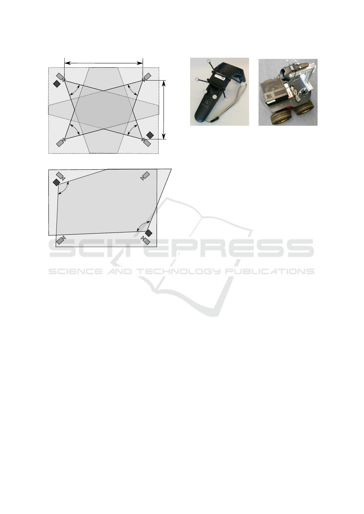
Figure 7: Camera setup for the multi-view and the dual-axis
rotating laser sweeps system.
Lighthouse system will be evaluated regarding track-
ing volume, accuracy, and applicability for mobile
robots.
7.2 Experimental Setup
To evaluate the possible accuracy of the HTC Light-
house system, an HTC Vive controller is equipped
with an optically trackable rigid body. The rigid body
is tracked by four Optitrack Prime 13 cameras. The
cameras have a horizontal fov of 56
◦
and a vertical
fov of 46
◦
. The laser planes of the HTC Vive light-
house emitter have a vertical and horizontal fov of
110 degrees. Figure 7 illustrates the camera placing
including the opening angle of the different tracking
solutions in a top-down view.
The setup for tracking the HTC Vive controller is
presented in Figure 8. A rigid body consisting of six
infrared marker is attached to the HTC Vive controller
to validate the tracked trajectory’s accuracy. In a sec-
ond experiment, the controller is fixed on the Pioneer
2 robot to measure the robot’s movement.
(a) Rigid setup of an HTC
Vive controller and an opti-
cally trackable rigid body.
(b) Pioneer 2 Robot with at-
tached trackable device ac-
croding to Figure 8(a).
Figure 8: Tracked controller device and robot platform as
used for evaluation.
7.3 Calibration
The tracking information of the HTC Vive is extracted
using the Valve OpenVR library which merges the
pose estimation based on the rotating laser sweeps
with additional measurements of an inertial measure-
ment unit.
The homogenous transformations X between the
rigid body and the controller and Z between the in-
frared marker coordinate system and the dual-axis
laser sweep coordinate system (see Figure 9) can be
computed by solving the following equation:
A
i
X = ZB
i
R
ai
t
ai
0 1
R
x
t
x
0 1
=
R
z
t
z
0 1
R
bi
t
bi
0 1
.
(20)
The rotational and translational part in Equation 20
can be rearranged in the linear system:
R
ai
⊗R
bi
−I
9
0
9×3
0
9×3
0
3×9
I
3
⊗t
T
bi
−R
ai
I
3
vec(R
x
)
vec(R
z
)
t
x
t
z
=
0
9×1
t
ai
.
(21)
Filling the position and orientation data from the
measurement systems into A
i
(HTC Vive Lighthouse)
and B
i
(Optitrack), Equation 21 can be solved in
the least-square sense. Notice, that the controller
has to undergo at least two independent general mo-
tions with nonparallel axes to retain a unique solu-
tion. Calibration was performed on 1000 measured
poses within a sphere diameter of 70.46 mm. The
overall mean pose error was 0.892 mm and 0.423
◦
.
With X and Z known, the following trajectories could
be transformed into the same coordinate system and
their position and rotation errors are calculated.
Tracking Solutions for Mobile Robots: Evaluating Positional Tracking using Dual-axis Rotating Laser Sweeps
161
Prime 13
Lighthouse
emitter
HTC
controller
IR
marker
rigid
body
A
i
B
i
X
Z
Figure 9: Geometric relation between the tracking Z and
the rigid body X coordinate systems. A
i
,B
i
: Time varying
measurement data.
7.4 Indoor and Outdoor Suitability
As an end consumer product for entertainment appli-
cations, the HTC Lighthouse is developed for indoor
usage. Based on the expected interference due to di-
rect sunlight, the photosensor signals will be strongly
affected by noise. Additionally, a clear detection of
the passing laser sweeps will probably not be possi-
ble in the presence of sunlight. Therefore, the system
is not suited for outdoor applications.
7.5 Measurement Rate
The laser planes of the HTC Lighthouse rotate at
3600 r pm. Thus, a full rotation takes 16.66 ms. One
laser sweep is completed in a half rotation and there-
fore takes 8.333 ms. The possible measurement rate
for considering both sweeps of one emitter results in
60 Hz. Updating the pose every sweep, the update
rate increases to 120 Hz. Because the sensor fusion
algorithm implemented in the OpenVR library also
uses an additional IMU for pose estimation, the re-
sulting update rate is higher after sensor fusion.
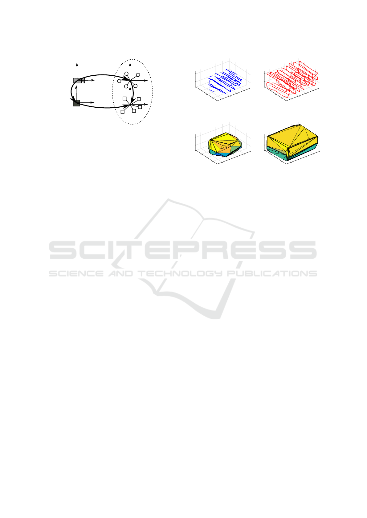
7.6 Tracking Volumes
We determine the trackable volume by manually mov-
ing the tracked device within the measurement se-
tups along the trajectory shown in Figure 10. The
trajectory is grid-like to receive a good coverage of
the volume. Since the illustration in Figure 10 only
shows the received pose data from the measurement
systems, gaps are indicating uncovered areas. As ex-
pected by the theoretical tracking area presented in
Figure 7, the object could be tracked more robust and
inside a larger volume using the HTC lighthouse sys-
tem. Whereas the rigid body needs to be visible in
at least two camera images to be tracked, the posi-
tion of the controller can be computed only visible
for one Lighthouse emitter. In contrast, the optical
1
2
z
2
1
1
y
0
x
0
-1
-1
-2
(a) Optitrack Prime 13.
1
2
z
2
1
1
y
0
x
0
-1
-1
-2
1
(b) HTC Lighthouse.
Figure 10: Measured trajectories of the different setups.
1
2
z
2
1
1
y
0
x
0
-1
-1
-2
(a) Optitrack Prime 13:
V
ot
= 10.22 m
3
.
1
2
z
2
1
1
y
0
x
0
-1
-1
-2
(b) HTC Lighthouse:
V
lh
= 27.02 m
3
.
Figure 11: Convex tracking volume of the different setups.
system is more robust against occlusions supporting
multiple points of view.
Figure 11 illustrates the tracking volume of the
Optitrack Prime 13 cameras and the HTC Lighthouse
systems. To get a measurable value to compare both
systems, the convex volumes around the trajectories
were calculated. Thereby we assume that the space
within the trajectory-grid is measurable as well.
Comparing both volumes, we see that the HTC
Lighthouse system is covering almost three times as
much volume as the Optitrack system. That ratio is no
constant value for all possible setups but underlines
the effect for setups with limited space and cameras.
7.7 Accuracy
To determine the static and dynamic accuracy, the
tracked device has been rigidly mounted on a Pioneer
2 robot. The resulting setup is shown in Figure 8. It
must be taken into consideration that the quality of
the calibration of Section 7.3 affects the dynamic and
static trueness.
Static Accuracy: To determine the static accuracy,
the robot has been placed statically on different posi-
tions inside the tracking volume near the center. The
trueness and precision have then been computed, us-
ing the tracking information of the Optitrack Prime 13
setup as ground truth. The static accuracy is given in
Table 1.
Dynamic Accuracy: The dynamic accuracy has been
computed controlling the robot manually on the tra-
jectories shown in Figure 12. As for the static accu-
racy, the Optitrack Prime 13 measurements are uses
as ground truth.
Table 1 shows the precision and trueness of the
ICINCO 2017 - 14th International Conference on Informatics in Control, Automation and Robotics
162
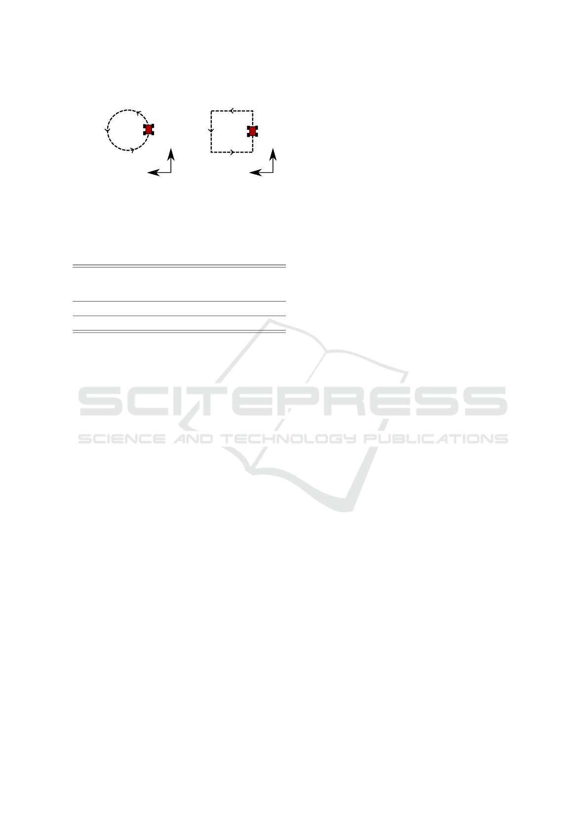
x
y
(a) Circle trajectory.
x
y
(b) Square trajectory.
Figure 12: Experimental trajectories.
reconstructed trajectories tracked by the Optitrack
Prime 13 setup and the HTC Lighthouse.
Table 1: Static and dynamic accuracy
Position
trueness
[mm]
Position
precision
[mm]
Orientation
trueness[
◦
]
Orientation
precision[
◦
]
Static 1.699 0.361 0.353 0.008
Dynamic 1.615 0.433 0.291 0.046
Results: With a position trueness of 1.615 mm
(static) and 1.699 mm (dynamic), the results are simi-
lar to the results given in (Burdea and Coiffet, 2003),
which declare an RMS of 1.0 mm at a distance of
1.0 m for the similar Laserbild 2 system. Consider-
ing the larger average distance between the emitter
and the tracking device in our setup, the measured ac-
curacy also increases as expected. The dynamic and
static position trueness are of a comparable magni-
tude. This can be reasoned by the relatively low speed
of the robot compared to the measurement rate of the
system.
8 CONCLUSION
In the first part of this paper, optical, acoustic, mag-
netic and inertial systems are compared regarding
their principle of function. A summarizing compar-
ison is given in Table 2.
The usage of the different tracking technologies
strongly depends on the application which the sys-
tem is needed for. Besides their line-of-sight limita-
tion, optical tracking systems are proofed to be robust
and to have a high accuracy. That is why stereo and
multi-camera systems are typically used for commer-
cial motion capture systems and are the standard in
clinical applications (Birkfellner et al., 2008). Based
on the widespread of mono cameras in handheld de-
vices as smartphones, fiducial markers are currently
state of the art for AR-applications. To improve the
accuracy of these systems further, the results of fidu-
cial marker tracking are often combined using sensor
fusion techniques with IMU data which are also state
of the art in smartphone applications.
Magnetic tracking systems use AC or DC field
coupling between source and sensor to determine the
transformation between them. Therefore, no line-of-
sight is required. As a restriction, magnetic systems
are susceptible to conductive and ferromagnetic mate-
rials. The resulting magnetic field distortions worsen
the trueness. A high resolution and precision can be
obtained, but decreases rapidly with the distance.
Acoustic systems based on the duration of ultra-
sonic waves are too inaccurate to be used for accurate
motion tracking. They are used in applications which
do not require a high accuracy as in basic indoor nav-
igation.
Inertial Systems are infrequently used as stand
alone tracking solutions based on the occurring drift.
Due to their low price microelectromechanical IMUs
are often used as additional sensors.
Laser-based optical systems using rotating laser
planes systems do have advantages, especially for vir-
tual reality applications because of the high measure-
ment rate and the low latency time (which is necessary
to avoid motion sickness) and the possibility to realize
position and orientation tracking on the same printed
circuit board. Therefore, no additional time synchro-
nization effort is necessary compared to combined de-
vices for orientation and position tracking, such as ex-
ternal multi-view systems. In contrast to other optical
systems, the usage of laser tracking based systems is
less flexible, based on the higher marker complexity.
Also, post processing is necessary to compute the po-
sition and the orientation based on the photodiode sig-
nals.
In the second part of this paper, it has been shown
experimentally, that pose tracking using dual-axis ro-
tating laser sweeps is a tracking solution which can
cover a large tracking volume only using a small
number of emitters. The experimentally evaluated
static and dynamic accuracy is lower than the accu-
racy which can be achieved by commercial multi-
camera setups. Nevertheless, the possible accuracy
of the HTC Lighthouse system can be considered to
be sufficient for many robotic applications.
REFERENCES
Abawi, D. F., Bienwald, J., and Dorner, R. (2004). Accu-
racy in optical tracking with fiducial markers: An ac-
curacy function for artoolkit. In Proceedings of the
3rd IEEE/ACM International Symposium on Mixed
and Augmented Reality, ISMAR ’04, pages 260–261,
Washington, DC, USA. IEEE Computer Society.
Tracking Solutions for Mobile Robots: Evaluating Positional Tracking using Dual-axis Rotating Laser Sweeps
163
Table 2: Comparison of the presented methods.
Method Typical Field of Application Advantages Disadvantages
Optical augmented reality applications inexpensive, line-of-sight necessary,
Single View simple setup small tracking volume
Optical instrument tracking in high accuracy line-of-sight necessary,
Stereo View medical applications small tracking volume
Optical motion capturing systems, high accuracy, line-of-sight necessary,
Multi View deformation analysis less occlusions expensive
Optical mobile robotics, head tracking, high accuracy line-of-sight necessary,
Laser virtual reality applications onboard processing required,
tracked device needs additional electronics
Magnetic body motion tracking, instrument inexpensive, no affected by magnetic interference,
tracking in medical applications line-of-sight necessary tracked device needs additional electronics
Acoustic rough localization using beacons, inexpensive low accuracy, low measurement rate,
underwater localization affected by ultrasonic interference,
tracked device needs additional electronics
Inertial supplement to other applications tracking volume not position highly affected by drift,
applications using sensor fusion limited, inexpensive, tracked device needs additional electronics
small, high
measurement rate
Andrew D. Wiles, D. G. T. and Frantz, D. D. (2004). Accu-
racy assessment and interpretation for optical tracking
systems. In In Medical Imaging 2004: Visualization,
Image-Guided Procedures, and Display, Vol. 5367 pp.
421-432.
Ascension Technology Corporation (2000). laserbird 2 -
precision optical tracking. Internet.
Bergamasco, F., Albarelli, A., Rodol, E., and Torsello, A.
(2011). Rune-tag: A high accuracy fiducial marker
with strong occlusion resilience. In CVPR, pages 113–
120. IEEE Computer Society.
Birkfellner, W., Hummel, J., Wilson, E., and Cleary, K.
(2008). Image-Guided Interventions, chapter Track-
ing Devices, pages 23–44. Springer-Verlag.
Burdea, G. C. and Coiffet, P. (2003). Virtual Reality Tech-
nology. John Wiley and Sons. Inc.
Hightower, J. and Borriello, G. (2001). Location systems
for ubiquitous computing. Computer, 34(8):57–66.
Hu, C., Meng, M.-H., and Mandal, M. (2007). A linear al-
gorithm for tracing magnet position and orientation by
using three-axis magnetic sensors. IEEE Transactions
on Magnetics, 43(12):4096–4101.
Islam, S., Ionescu, B., Gadea, C., and Ionescu, D. (2016).
Indoor positional tracking using dual-axis rotating
laser sweeps. In 2016 IEEE International Instrumen-
tation and Measurement Technology Conference Pro-
ceedings, pages 1–6.
Mikko Kyt, Mikko Nuutinen, P. O. (2011). Method for mea-
suring stereo camera depth accuracy based on stereo-
scopic vision. In Three-Dimensional Imaging, Inter-
action, and Measurement, Conference Volume 7864.
Noriega-Manez, R. J. (2007). Inertial navigation. Course-
work for Physics 210, Stanford University, Autumn
2007.
NovAtel (2014). Imu errors and their effects. APN-064.
Paperno, E., Sasada, I., and Leonovich, E. (2001). A new
method for magnetic position and orientation track-
ing. IEEE Transactions on Magnetics, 37(4 I):1938–
1940.
Pentenrieder, K., Meier, P., Klinker, G., and Gmbh, M.
(2006). Analysis of tracking accuracy for single-
camera square-marker-based tracking. In Proc. Drit-
ter Workshop Virtuelle und Erweiterte Realit
¨
at der GI-
Fachgruppe VR/AR, Koblenz, Germany.
Polhemus, I. (2017a). Fastrack - the fast and easy
digital tracker. Internet. http://polhemus.com/
assets/img/FASTRAK Brochure.pdf.
Polhemus, I. (2017b). Patriot wireless. Inter-
net. http://polhemus.com/ assets/img/ PA-
TRIOT WIRELESS brochure.pdf.
Priyantha, N. B., Chakraborty, A., and Balakrishnan, H.
(2000). The cricket location-support system. In Pro-
ceedings of the 6th Annual International Conference
on Mobile Computing and Networking, pages 32–43.
Raab, F., Blood, E., Steiner, T., and Jones, H. (1979). Mag-
netic position and orientation tracking system. In
IEEE Transactions on Aerospace and Electronic Sys-
tems, volume 15.
Szeliski, R. (2010). Computer Vision: Algorithms and
Applications. Springer-Verlag New York, Inc., New
York, NY, USA, 1st edition.
Ward, A., Jones, A., and Hopper, A. (1997). A new location
technique for the active office. IEEE Personal Com-
mun., 4(5):42–47.
Woodman, O. J. (2007). An introduction to inertial naviga-
tion. Technical Report UCAM-CL-TR-696, Univer-
sity of Cambridge, Computer Laboratory.
ICINCO 2017 - 14th International Conference on Informatics in Control, Automation and Robotics
164
