Index Clustering: A Map-reduce Clustering Approach using Numba

Xinyu Chen and Trilce Estrada

University of New Mexico, Albuquerque, U.S.A.

Keywords:

Scalable Clustering, Privacy Preserving, Big Data.

Abstract:

Clustering high-dimensional data is often a crucial step of many applications. However, the so called ”Curse

of dimensionality” is a challenge for most clustering algorithms. In such high-dimensional spaces, distances

between points tend to be less meaningful and the spaces become sparse. Such sparsity needs more data

points to characterize the similarities so more distance comparisons are computed. Many approaches have

been proposed for reduction of dimensionality, such as sub-space clustering, random projection clustering,

and feature selection technique. However, approaches like these become unfeasible in scenarios where data is

geographically distributed or cannot be openly used across sites. To deal with the location and privacy issues

as well as mitigate the expensive distance computation, we propose an index-based clustering algorithm that

generates a spatial index for each data point across all dimensions without needing an explicit knowledge of

the other data points. Then it performs a conceptual Map-Reduce procedure in the index space to form a ﬁnal

clustering assignment. Our results show that this algorithm is linear and can be parallelized and executed

independently across points and dimensions. We present a Numba implementation and preliminary study of

this algorithm’s capabilities and limitations.

1 INTRODUCTION

Clustering technology has been challenged by the

rapid growing of data. In domains where data vol-

ume is continuously growing (e.g., climate simula-

tions - 32 PB, astronomy - 200 GB/day to 30 TB/day,

and high-energy physics - 500 EB/day), data move-

ment and centralized processing represent perfor-

mance bottlenecks that increase resource pressure on

storage, bandwidth, memory, and CPU (Tiwari et al.,

2012). The problem becomes even more challenging

as the number of distributed locations increases, or as

privacy and management impose restrictions to data

access. Two scenarios are of relevance for this work:

(1) In-situ data analysis of HPC simulations. Anal-

ysis has to be done on site, using local data, in real

time, along with as little communication as possible.

(2) Medical data analysis. Data volume may not be

too large to be efﬁciently moved across locations, but

privacy issues may restrict data sharing. In both sce-

narios, a global model has to be computed at run time

using only an incomplete view of the data. Our ques-

tion is if data cannot be moved, or shared, how can

we still learn from it?.

From the standpoint of scalability in parallel and

distributed environments and privacy bound applica-

tions, state of the art clustering techniques lack in one

or more of the following crucial aspects: (1) Tradi-

tional machine learning and data mining approaches

rely on expensive training phases and often require

gathering data in a centralized (

ıma and Orponen,

2003), (Salakhutdinov and Hinton, 2009) or semi-

centralized (Kargupta et al., 2001), (Boyd et al., 2011)

way. (2) Existing distributed approaches either re-

quire synchronized communication (Bandyopadhyay

et al., 2006), are tied to a particular domain and do not

generalize (Estrada and Taufer, 2012), (Kawashima

et al., 2008), sacriﬁce accuracy for the sake of scala-

bility (Liu et al., 2013), (Gionis et al., 1999), (Aggar-

wal et al., 1999), or are affected by the curse of dimen-

sionality (Quiroz et al., 2012) (i.e., scaling the num-

ber of data features negatively affects an algorithm’s

predictive capabilities (Indyk and Motwani, 1998)).

None of these methods are all, scalable, accurate, and

general enough to be useful in privacy bound or dis-

tributed scenarios of Big Data.

Our goal is to build a clustering algorithm that is

able to organize large dimensional datasets without

relying on a global knowledge of the data or expen-

sive distance computations. This is a key step that

may eventually lead to a solution for location and pri-

vacy restricted situations: the clustering can be done

locally on each distributed site by exchanging only

summarized information, like bins and frequencies,

Chen, X. and Estrada, T.

Index Clustering: A Map-reduce Clustering Approach using Numba.

DOI: 10.5220/0006437402330240

In Proceedings of the 6th International Conference on Data Science, Technology and Applications (DATA 2017), pages 233-240

ISBN: 978-989-758-255-4

233

with other sites. Compared to moving the whole raw

dataset around, the summarized information is ex-

tremely small. Individual data points cannot be repro-

duced from such limited information on other sites so

that the privacy is well protected. With this in mind,

we propose Index Clustering, a new data clustering

approach based on indexing individual data points

across their whole high dimensional space, and then

using only the indexes to build ﬁnal clusters. Without

distance computation, our algorithm has a linear time

complexity with regards to both the number of points

and dimensions. More speciﬁcally, the processing of

each point can be done in a constant time. Finally, un-

like most density-based clustering methods, our algo-

rithm can beneﬁt from a large number of dimensions.

This paper’s contributions are as follow:

• A linear time complexity clustering approach that

is able to group data across multiple dimensions

even with a very limited view of the data.

• A parallel implementation of our algorithm in

GPU using Numba.

• A preliminary evaluation of our algorithm’s scal-

ability and generality using synthetic and real

datasets.

The remainder of this paper is organized as fol-

lows: in section 2, we brieﬂy summarize some algo-

rithms that have inﬂuence on our algorithm as well

as other related approaches. Section 3 presents our

index-based clustering algorithm, which combines a

map-reduce like approach with Numba to accomplish

the parallel clustering tasks. In section 4 we explain

the experimental results. Section 5 presents our dis-

cussion regarding our algorithm’s limitations, reason-

ing behind parameter selection, and overview of fu-

ture works that can improve the robustness of our

method. Finally, section 6 concludes the paper.

2 RELATED WORK

Scalable methods, closely related to our techniques,

are density-based clustering. One of the ﬁrst ap-

proaches is DBSCAN (Ester et al., 1996). Another

successful example is the Decentralized Online Clus-

tering (Quiroz et al., 2012) that was used in the con-

text of distributed systems monitoring and resource

provisioning. Our approach is similar to these tech-

niques in the sense that it groups points in a density-

based way; but it is different in that we use indexed

bins to deﬁne dense regions that contain enough

points instead of deﬁning some core points that have

enough neighbors.

Other methods have been proposed to capture

low-dimensional semantics of data features with the

ﬁnal purpose of accelerating searches for similar

items. Successful methods in this category include

Latent Semantic Analysis (LSA), Semantic Hashing,

and Lazy Learning (Indyk and Motwani, 1998; Bar-

rena et al., 2010; Omercevic et al., 2007). Latent Se-

mantic Analysis (Deerwester et al., 1990) uses the

SVD decomposition to extract low dimensional se-

mantic structure of the word-document co-occurrence

matrix. LSA enables document retrieval engines to

base their searches on semantic structure, rather than

using individual word counts. This property greatly

reduces the time complexity of the algorithms. How-

ever, computing the SVD decomposition becomes un-

feasible as data size grows large.

Sub-space Clustering algorithms gave inspi-

ration to our algorithm. Grid-based hierarchi-

cal clustering algorithms that use bottom-up search

strategies are most related and inﬂuential to us.

CLIQUE (Agrawal et al., 1998) and MAFIA (Goil

et al., 1999) ﬁrst ﬁnd dense regions in lower-

dimensional spaces. Then they merge these lower-

dimensional regions into bigger higher-dimensional

hyper-cubes if they can ﬁnd a common-face between

two regions. The limitation of these two algorithms

is the expensive combinations of all possible lower

dimensional regions so they didn’t show scalability

when the dimensionality goes to several hundred.

3 ALGORITHM

Most traditional clustering techniques rely on com-

puting pairwise distances between points or regions

to form clusters. These computations are exponen-

tially expensive as the number of points and the num-

ber of dimensions grow. Other more efﬁcient tech-

niques such as dimensionality reduction, need prior

knowledge of the data (e.g. its principal components,

covariance matrix, or some other statistical proper-

ties). However, when data needs to be analyzed as a

stream, in situ, or on different geographical locations,

and the i.i.d.(independent and identically distributed)

property cannot be guaranteed, then these methods

fail.

For an algorithm to work in such circumstances,

the main question is: if we cannot compute pairwise

distances, how can we decide whether two points are

similar? To efﬁciently answer this question, we took

inspiration from Locality Sensitive Hashing (Gionis

et al., 1999). Similar to the family of hashed val-

ues, we map data points to indexes along every di-

mensions. By organizing these indexes into bins and

DATA 2017 - 6th International Conference on Data Science, Technology and Applications

234

merging bins to primary clusters, we get a list of pri-

mary cluster identiﬁers like the ﬁngerprints for each

point which we call it a index. Then, forming clus-

ters can be done in this projected space, and is al-

most as easy as performing a reduction on ﬁnger-

prints. The A-priori algorithm for mining frequent

patterns (Agrawal et al., 1994) is behind our ﬁnal

grouping approach: Points belong to one higher di-

mensional cluster also stay together in each lower di-

mensional regions; Points with different ﬁngerprints

belongs to different clusters. Two crucial aspects of

this process are: (1) the space of indexes represents

summarized knowledge of the raw data, which allows

us to preserve privacy, and (2) the reduction on ﬁnger-

prints instead of distance comparisons, which allows

us to improve scalability.

3.1 Methods

We want to cluster a dataset m of size M × N, where

M is the number of data points and N is the number of

features. We denote m = {cor

i, j

|i < M, j < N}, with i

being the unique identity of a data point and j its jth

feature. Without lack of generality we could assume

M = 1 for a data stream scenario or multiple m’s for a

distributed case. For descriptive purposes we will call

m as our raw data for the rest of the paper. The steps

of our method are as follows:

1. Assign a list of indexes to a point. Every index

is associated with a bin in the speciﬁc dimension.

As points get their indexes, bins update their den-

sity. This step only involves the point itself and

the value range of each dimension. In the dis-

tributed scenario this can be done with only local

data.

2. Building primary clusters. A primary cluster is

a partial clustering assignment viewed from one

particular dimension. This step merge adjacent

bins into what we call primary clusters if they ex-

ceed the density threshold.

3. Assigning points to ﬁnal clusters. Once primary

clusters are built, every point can be mapped to a

speciﬁc set of primary clusters in all of its dimen-

sions. They use their indexes to get a index. This

leads to a ﬁnal global clustering assignment.

3.1.1 Assigning a List of Indexes to a Point

A point

’s coordinate are converted to idx, a list of

indexes indicating a relative location along each di-

mension. The number of bits per index is deﬁned by

the user as the depth of our algorithm. This depth

also determines the number of bins per dimension as

B = 2

depth

. Then, idx

i, j

, which is the index for x

i, j

in range of [0,2

depth

− 1].

The function getindex as shown in Algorithm 1,

receives as parameters the depth of indexes, an es-

timated lower and upper boundaries of the speciﬁc

dimension, and the point’s coordinate. Then, it recur-

sively divides the range on one dimension into equal

halves for depth number of steps. This procedure is

conceptually building a depth deep binary tree to ac-

commodate the range. Each leaf contains a sub re-

gion of the bounded dimension. The point’s coordi-

nates are then converted into indexes of leaves. The

getindex function is applied to x

i, j

∀i, j independently.

Thus, it can be efﬁciently implemented in parallel, not

only per data point but also per feature.

Algorithm 1: getindex.

1: procedure GETIDX(max depth,lower,upper,x

i, j

)

2: for depth < max depth do

3: µ

j,depth

← 1/2(lower + upper)

4: if x

i, j

≥ µ

j,depth

then

5: append 1 to idx

i, j

6: lower ← µ

j,depth

7: else

8: append 0 to idx

i, j

9: upper ← µ

j,depth

10: return idx

i, j

 return leaf index

3.1.2 Building Primary Clusters

Primary clusters are sets of bins organized in a par-

tial clustering assignment for a single dimension.

Our algorithm follows a bottom-up strategy. Un-

like CLIQUE(Agrawal et al., 1998) and MAFIA(Goil

et al., 1999), we build primary clusters on each di-

mension then directly reduce to the entire dimensional

clusters and skip all intermediate lower-dimensional

dense regions. A bin is instantiated only when there

is a data point whose index on this dimension is as-

sociated to that bin. bins = {dbin

b, j

|b < B, j < N}.

dbin

b, j

is the density of bin b on the jth dimension.

To build primary clusters we merge adjacent bins

if their density is larger than a predeﬁned threshold

minDensity. For very sparse clustering, this thresh-

old can be set to zero. A primary cluster represents

an agglomeration of points viewed from one particu-

lar dimension. We refer them as pc where {pc

b, j

|b <

B, j < N} contains a unique identiﬁer (e.g. PCid) for

the primary cluster in that dimension, with B and N

being the number of bins and the number of dimen-

sions respectively. Algorithm 2 shows the procedure

for building primary clusters. A while loop for gener-

ating point’s indexes and updating bins’ density, and

a for loop for merging adjacent bins forming primary

Index Clustering: A Map-reduce Clustering Approach using Numba

235

clusters. The only communication needed would be

the ﬁnal bin densities, which is considerably smaller

than raw data and has no sensitive information that

could compromise privacy.

Algorithm 2: Build Primary Clusters.

1: M = numberOfPoints

2: N = numberOfDimension

3: minD = minimumDensityInBin

4: depth = depthOﬁndex

5: B = 2

depth

numberOfBins

6: while not EOF do  generate indexes, ﬁll bins

7: cor ← one data point from raw data

8: idx ← getindex(depth, cor)

9: for j = 1 to N do

10: dbin

j,idx

+ = 1  increase bin density

11: PCid ← 0  initialize for noise

12: for i = 1 to N do  merge bins

13: k ← 1, f lag ← f alse

14: while k ≤ B do

15: if dbin

i,k

> minD AND not f lag then

16: PCid ← k

17: f lag ← true

18: else if dbin

i,k

<= minD AND f lag then

19: PCid ← 0

20: f lag ← f alse

21: pc

i,k

← PCid

22: k ← k + 1

3.1.3 Assigning Points to Final Clusters

The ﬁnal step makes a ﬁnal assignment of points to

their respective clusters. The aggregated clusters are

represented as FC = { f c

|m < M}. The index for a

ﬁnal cluster is just the concatenation of PCids of each

one-dimensional primary cluster. The intuition being

that if points belong together in a high dimensional

cluster, they will be together with high frequency in

lower dimensional clusters. Although the possible

combination of primary cluster indexes is vast, the

real worst case is each point forms a unique ”group”.

So we can bound the maximum number of ﬁnal clus-

ters to be M. Algorithm 3 shows the procedure of

building ﬁnal clusters. This procedure consists on

concatenating the set of primary clusters assigned to

a point to build a global index which determines the

point membership to a speciﬁc ﬁnal cluster.

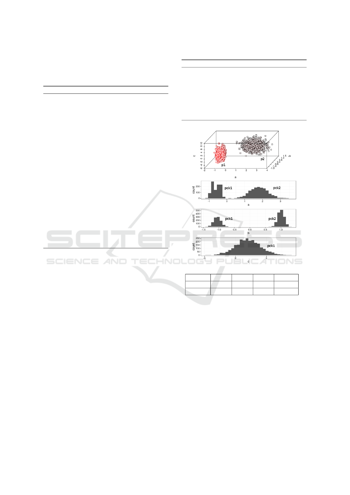
In ﬁgure 1(a) we illustrate the algorithm with an

intuitive example. Two primary clusters are formed

on dimension

,dimension

, and one primary cluster

forms on dimension

. Final clusters are built upon

points sharing the same concatenation of their PCids.

, p

are from the red and black group respectively.

Figure 1(b) shows their speciﬁc primary clusters

Algorithm 3: Final clustering.

1: M = numberOfPoints

2: N = numberOfDimensions

3: pc = primaryClusters

4: for i = 1 to M do  concatenate PCids

5: for k = 1 to N do

6: fcindex ← concatenate pc

i,k

7: f c

f cindex

+ = 1  increase cluster density

(a) 2 ﬁnal clusters and bin densities.

pointID PCid

PCid

fcindex

1 1 1 111

2 2 1 221

(b) Example of primary clusters and ﬁnal clusters in-

dexes

Figure 1: Didactic example of how our algorithm will

merge adjacent bins into primary clusters and reduce on

PCids to form a global arrangement.

across the three dimensions. The column fcindex

shows their ﬁnal clustering assignments. Note that

with this arrangement, it is very easy to collapse a par-

ticular dimension and form completely different clus-

tering assignments without having to reiterate through

the data.

3.2 Parallel Implementation with

Numba

We used Numba to accelerate the above algorithm.

Numba is an Open Source NumPy-aware optimizing

compiler for Python that generates machine code for

DATA 2017 - 6th International Conference on Data Science, Technology and Applications

236

both CPUs and NVIDIA GPUs. To Assign indexes

is the most time consuming section. We parallelized

the function getindexGPU and ﬁllBinsGPU with one

GPU thread per coordinate. To build primary clusters,

the buildPClustersGPU function is implemented in a

limited parallel manner. The algorithm only launches

one thread per dimension. The location to merge bins

starts from the lowest bin. Since this step is not the

most computationally expensive in our method, we

leave it in a simple parallel approach. The Numba

sequence of steps is described in Algorithm 4.

Algorithm 4: Parallel map-reduce clustering algorithm.

1: M = numberOfPoints

2: N = numberOfDimension

3: B = numberOfBins

4: wt ← rand(w

,...,w

)

∈ (0,1)

5: m ← readFile  get cor

i, j

6: k ← getindexGPU  get idx

i, j

7: dbin ← ﬁllBinsGPU  get dbin

i,k

8: pc ← buildPClustersGPU  get pc

i,k

9: cg ← getPrimaryClusterindex  additional step

10: cm ← cg · wt  additional step

11: ck ← getindexGPU  additional step

12: hc ← ﬁllBinsGPU  additional step

13: for i = 1 to M do  output ﬁnal clusters

14: if hc

f cindex

≥minThreshold then

15: output ﬁnal cluster

f cindex

The current version of Numba has no direct string

operations. Our implementation uses four additional

steps (lines 9 to 12 in Algorithm 4) to accomplish

the ﬁnal clustering assignment. To emulate the se-

rial implementation of concatenating each of the pri-

mary cluster indexes in a point’s dimensions, we

ﬁrst fetch the primary cluster indexes into a ma-

trix cg = {cid

i, j

|i < M, j < N}. Then we multiply

c with a random N dimensional real vector wt =

,...,w

)

∈ (0,1). The result is a column

vector cm = {hk

|i < M}. So we get an unique real

number hk

to replace the concatenation of primary

cluster indexes. We will discuss the correctness of

this later in section 5.

The above two steps generate a 1 dimensional

array of real number ﬁnal cluster indexs for every

points. We use an additional generate index step to

scatter these indexes onto a deeper binary tree. This

converts the vector cm = {hk

∈ R} of real numbers

into the integer vector ck = {ck

∈ I} with unique in-

tegers per bin. Our worst case is still when each point

has an unique ﬁnal cluster index. To assure each of

the resulting leaf indexes are unique, the additional

getindex step uses a new depth > log(M). The last

additional step consists on keeping track of the den-

sity of bins in ck.

3.3 Time Complexity

In Algorithm 1, getindex uses a constant depth steps

to convert coordinates to indexes. The while loop

in Algorithm 2 goes one pass through all M points

to convert coordinates to indexes and accumulate the

bin densities on all N dimensions. This pass will be

O(M × N). The for loop goes one pass through bins

on N dimensions to merge them into Primary Clus-

ters. The number of bins is 2

depth

. This adds up

to O(2

depth

× N). The Algorithm 3 goes through all

M points on all N dimensions adds up to O(M × N).

The overall time complexity will be O(M × N) +

O(2

depth

× N). Normally, we set depth to 10 to 15 so

M > 2

depth

. The time complexity is still O(M × N).

The Numba implementation can parallelize the above

computations to the number of GPU threads P. So

The overall time complexity reduces to O(M ×

As P and N are ﬁxed for a given dataset, our algorithm

can be seen as linear to the number of data points with

time complexity = O(M).

4 EXPERIMENTS AND RESULTS

We empirically evaluate the scalability and generality

of our Index Clustering algorithm through three tests.

First we compare performance between the serial and

the GPU implementations to quantify gains obtained

from the algorithm’s parallelization. Then, we per-

form controlled scalability tests to quantify perfor-

mance when we varied the number of points or the

number of dimensions. Finally, we use the algorithm

on real datasets to understand its predictive capabil-

ities. All the experiments ran on an 8 core Intel

Haswell 2.4GHz machine with a 640 Maxwell core

0.9GHz SMM graphic card. The host RAM is 8G and

the device RAM is 2G.

4.1 Performance Gain from GPU

Our ﬁrst experiment is to quantify the improvement of

performance of GPU parallelization. We used simple

synthetic data to allow us control over the dimension-

ality and size of the datasets. We used the data gen-

erator from gpumaﬁa(Canonizer, ) to generate 1 mil-

lion 20-dimensional points grouped into 5 hypercubic

clusters with 10% uniformly distributed noises. We

sum up the additional steps on the GPU implementa-

tion to get an equivalent timing for the ﬁnal clustering

step on CPU. Figure 2 shows the time for clustering

1 million 20 dimensional points into 5 groups. The

algorithm successfully found ﬁve groups with recall

and precision equal to 1.0. The GPU implementation

Index Clustering: A Map-reduce Clustering Approach using Numba

237

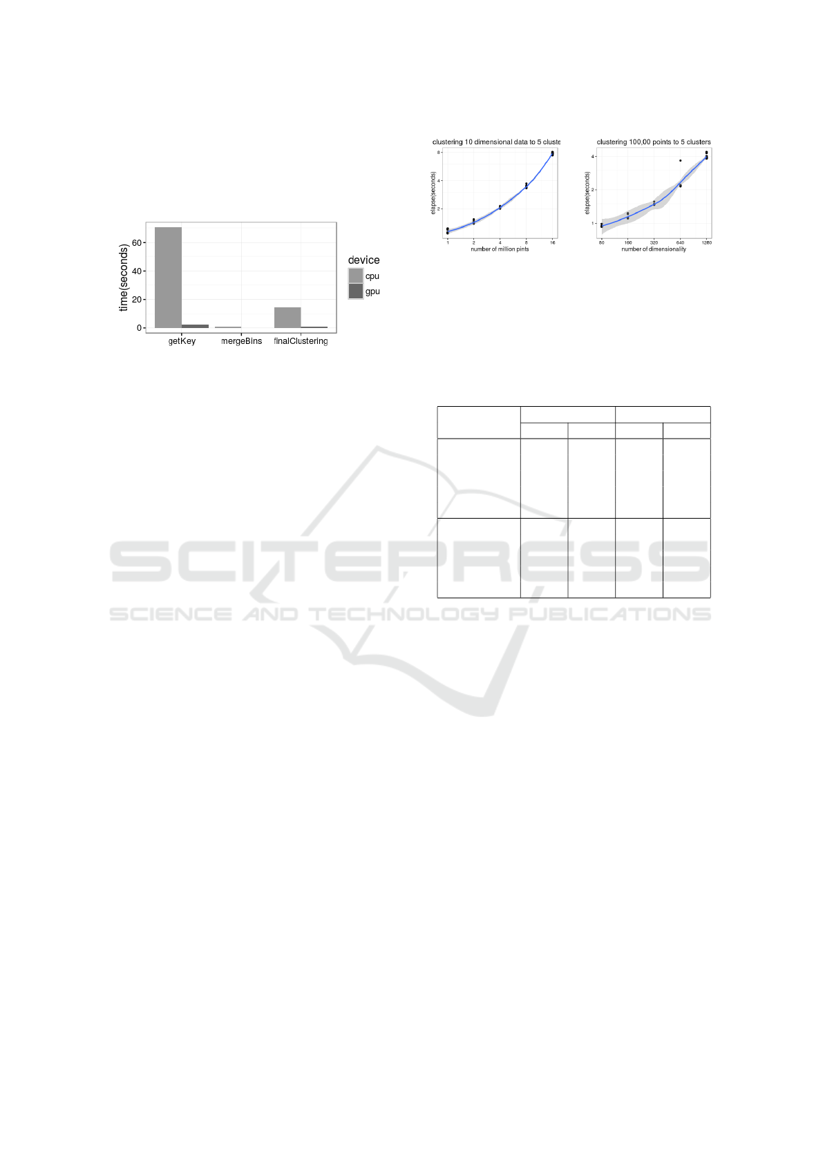
is about 30 time faster than CPU. Performance is ex-

pected to plateau as the number of data dimensions

approach the maximum number of threads. However,

this is a limitation of the hardware rather than of the

algorithm.

Figure 2: Elapsed time consumed by each step on CPU and

GPU in clustering 1 million low dimensional points.

4.2 Scalability

Our second set of experiments are designed to test the

algorithm’s weak scalability as the number of points

or the number of dimensions grow.

We ﬁrst ﬁxed the dimensions to 10 and number of

clusters to 6. Then we varied the number of points

from 1 million to 16 million with intermediate mea-

sures at 2, 4, and 8 million. Figure 3(a) shows the

relationship between time and size of the datasets is

close to linear. Through experimentation we observed

that the depth = 15 and minpt = 10 produced accu-

rate clusters for the 1 million dataset, and minpt = 100

for the 16 million dataset. Even though it is apparent

that the depth parameter is weakly correlated to the

data size, its relative growth is so small that it does

not have a considerable effect on the time complexity

of the algorithm.

Next we ﬁxed the number of points to 100,000 and

varied the number of dimensions from 80 to 1280(i.e,

80, 160, 320, 640, 1280). Again, the algorithm suc-

cessfully divided the points into 5 groups. Figure 3(b)

shows that the relationship between time and dimen-

sionality is close to linear.

4.3 Comparison with K-means

It’s better to compare with density-based algorithms.

However, DBSCAN failed to ﬁnish 1 million data

points due to its quadratic complexity. So we com-

pare our algorithm with the K-Means due to its high

performance and widely acceptance in many disci-

plines. We picked the implementation of K-means in

scikit-learn package 0.17.1. To avoid hardware dif-

ference, only accuracy is compared. We simply give

K-means the ground truth value of k. Table 1 con-

tains averaged recall and precision of 10 runs for each

row. This comparison shows the generated separa-

(a) Scalability as data

points increases

(b) Scalability as dimen-

sionality increases

Figure 3: Scalability as dataset size and dimensionality in-

crease. Above: time for clustering 10 dimensional data with

size of 1, 2, 4, 8,and 16 million points. Below: time for

clustering 100,000 points with 80, 160, 320, 640 and 1280

dimensions.

Table 1: Index Clustering (idxc) VS. K-Means (kms).

Recall Precision

idxc kms idxc kms

1m-10d 0.999 0.798 1.0 0.788

2m-10d 0.999 0.799 1.0 0.841

4m-10d 0.999 0.800 0.999 0.791

8m-10d 0.999 0.799 1.0 0.806

16m-10d 0.999 0.800 1.0 0.601

100k-80d 0.999 0.800 1.0 0.984

100k-160d 0.999 0.804 1.0 0.746

100k-320d 0.998 0.799 1.0 0.738

100k-640d 0.998 0.797 1.0 0.736

100k-1280d 0.996 0.801 1.0 0.741

ble boundaries of synthetic hypercubes help our al-

gorithm achieve high accuracy. But the pairwise dis-

tances trick K-Means to lower accuracy.

4.4 Clustering Real Data

We tested our algorithm on the Daily and Sports Ac-

tivities Data Set(Altun et al., 2010) from the UCI

Machine Repository. The data set contains 45-

dimensional signals measured from different physical

activities performed by eight persons.

The ﬁrst experiment is to identify different activi-

ties of the same person. We considered sitting, walk-

ing on a treadmill and jumping. Each activity contains

7,500 records. The total observations per person are

22,500. Without further preprocessing, our algorithm

separates the signals into three well deﬁned groups.

The algorithm discards a few observations (in the or-

der of 20 per person) as noise. However, it correctly

assigns 99.9% of the data to the correct activities.

The second experiment aims to identify differ-

ent people doing a particular activity. In this case

total 60,000 points per activity for 8 persons. Our

algorithm consistently identiﬁed nine distinct clus-

DATA 2017 - 6th International Conference on Data Science, Technology and Applications

238

ters. The nine-th cluster can be explained as noisy

inputs and inconsistencies of participants performing

the physical activity during the data collection.

5 DISCUSSION

In this section, we discuss the limitations of our algo-

rithm. This will help us to decide whether and when

the algorithm can accomplish its tasks.

Our algorithm works well with the assumption

that all dimensions are orthogonal to each other.

Adding one orthogonal dimension only stretches

points farther. However, adding one non orthogonal

dimension may compress points closer. To avoid this

problem, our algorithm makes it easy to collapse di-

mensions. If the collapse produces radically different

clustering assignments, it is possible to determine that

some dimensions are not orthogonal and need to be

revised.

Another limitation is the situation where the dense

bins of two clusters overlap. Figure 4 shows a com-

mon situation in a 2 dimensional space, where the

projected dense bins of cluster

and cluster

over-

lap on both dimensions. Our algorithm would fail

if they overlap in all dimensions. If p

is the prob-

ability of overlapping on the ith dimension, then the

probability that our algorithm fails is

∏

i=1

, which

becomes small quickly as dimensionality increases.

Thus, our algorithm is likely to perform better with

high dimensional data. To ameliorate the overlapping

problem, we can check dimension

in Figure 4 to ob-

serve a bimodal distribution of densities. An analy-

sis of the modes per range would give us indications

that the data is actually forming two clusters instead

of one. Again, as the number of dimensions increase,

the probability of successfully identifying this phe-

nomena just increases.

Unique Final Cluster indexes. In Section 3.2, we

convert the row vector of primary cluster into a real

value as the ﬁnal index. We accomplish this goal

by multiplying this row vector with a random col-

umn weight vector wt = (w

,..,w

)

∈ (0,1).

In Table 2, the column PCid

and PCid

are primary

cluster indexes. We can generalize the number of pri-

mary clusters in dimension

and dimension

to be X

and Y . The maximum number ﬁnal cluster indexes. is

X ×Y .

Let the weight vector be wt = (

a+1

) where a

is an integer and a · (a + 1) ≥ X ·Y . The dot product

of the matrix of PCids with wt is an 1-dimensional

column vector of real values. The results are within

the range of [

2a+1

a(a+1)

X(a+1)+aY

a(a+1)

]. The minimum step

between two values will be

a(a+1)

. This value range

Figure 4: Algorithm cannot separate two clusters when his-

tograms overlap on both dimensions. This happens more

often in lower dimensional spaces.

Table 2: Generate unique cluster indexes.

PCid

Weight Result

1 1 (1/2,1/3)

5/6

1 2 (1/2,1/3)

7/6

1 3 (1/2,1/3)

9/6

2 1 (1/2,1/3)

8/6

2 2 (1/2,1/3)

10/6

2 3 (1/2,1/3)

12/6

contains a(X + Y − 2) + X points. Solve the above

inequality we have a ≥

XY +

−

. Given X,Y,a

are all integers, we can simplify the inequality to be

a > min(X,Y ). This will give us the lower bounds of

the number of unique points XY + (X

− X),(X ≥ Y )

or XY + (Y

−Y ),(Y ≥ X ). For both cases, the lower

bound will be larger than the maximum number of

all possible ﬁnal cluster indexes. In the above ex-

ample, X = 2,Y = 3. We choose a = 2 such that

a(a + 1) ≥ XY . Then wt = (1/2,1/3)

. The result

ﬁnal cluster indexes are all unique. We can choose

wt = (

)

instead of (

a+1

)

as long as |a − b|

is still small, and a · b ≥ X · Y . Our algorithm uses

random real numbers within (0,1) to simulate such

a weight vector. For the purpose of querying a new

point’s cluster index, we can generate a ﬁxed weight

vector as the index generator.

6 CONCLUSIONS

In this paper we presented the Index Clustering algo-

rithm, a parallel clustering algorithm tailored for sce-

narios with very limited view of the data. Our algo-

rithm, is able to organize large dimensional datasets

without pair-wise point comparisons. This enables

us to form clusters under location and privacy re-

stricted situations. The communication is extremely

small compared to the whole raw dataset and indi-

Index Clustering: A Map-reduce Clustering Approach using Numba

239

vidual data points cannot be reproduced from it. Our

algorithm shows weak scalability with the number of

points/dimensions. The limitation of dimension or-

thogonality and overlapping is discussed. Such sit-

uation shall be rare as dimensionality grows higher.

Domain knowledge can beneﬁt our algorithm by pro-

viding guidelines for collapsing particularly noisy or

non-orthogonal dimensions. Finally, this work shows

the potential power of Numba in high-dimensional

data analysis.

ACKNOWLEDGEMENTS

This research was supported by the National Science

Foundation for the grant entitled CAREER: Enabling

Distributed and In-Situ Analysis for Multidimensional

Structured Data (NSF ACI-1453430).

REFERENCES

Aggarwal, C. C., Wolf, J. L., Yu, P. S., Procopiuc, C., and

Park, J. S. (1999). Fast algorithms for projected clus-

tering. SIGMOD Rec., 28(2):61–72.

Agrawal, R., Gehrke, J., Gunopulos, D., and Raghavan, P.

(1998). Automatic subspace clustering of high dimen-

sional data for data mining applications. ACM SIG-

MOD Record, 27(2):94–105.

Agrawal, R., Srikant, R., and Others (1994). Fast algo-

rithms for mining association rules. In Proc. 20th

int. conf. very large data bases, VLDB, volume 1215,

pages 487–499.

Altun, K., Barshan, B., and Tunc¸el, O. (2010). Comparative

study on classifying human activities with miniature

inertial and magnetic sensors. Pattern Recognition,

43(10):3605–3620.

Bandyopadhyay, S., Giannella, C., Maulik, U., Kargupta,

H., Liu, K., and Datta, S. (2006). Clustering dis-

tributed data streams in peer-to-peer environments. In-

formation Sciences, 176(14).

Barrena, M., Jurado, E., M

arquez-Neila, P., and Pach

on, C.

(2010). A ﬂexible framework to ease nearest neighbor

search in multidimensional data spaces. Data Knowl.

Eng., 69(1):116–136.

Boyd, S., Parikh, N., Chu, E., Peleato, B., and Eckstein, J.

(2011). Distributed optimization and statistical learn-

ing via the alternating direction method of multipliers.

Found. Trends Mach. Learn., 3(1):1–22.

Canonizer. Implementation of maﬁa subspace clustering on

nvidia gpus. https://github.com/canonizer/gpumaﬁa.

open source code 2012.

Deerwester, S., Dumais, S. T., Furnas, G. W., Landauer,

T. K., and Harshman, R. (1990). Indexing by latent

semantic analysis. Journal of the American Society

for Information Science, 41(6).

Ester, M., Kriegel, H.-P., Sander, J., Xu, X., and Others

(1996). A density-based algorithm for discovering

clusters in large spatial databases with noise. In Kdd,

volume 96, pages 226–231.

Estrada, T. and Taufer, M. (2012). On the effectiveness of

application-aware self-management for scientiﬁc dis-

covery in volunteer computing systems. In Proceed-

ings of the International Conference on High Perfor-

mance Computing, Networking, Storage and Analysis,

pages 80:1–80:11. IEEE Computer Society Press.

Gionis, A., Indyk, P., and Motwani, R. (1999). Similarity

search in high dimensions via hashing. In Proceedings

of the 25th International Conference on Very Large

Data Bases, pages 518–529. Morgan Kaufmann Pub-

lishers Inc.

Goil, S., Nagesh, H., and Choudhary, A. (1999). MAFIA:

Efﬁcient and scalable subspace clustering for very

large data sets. . . . Discovery and Data Mining,

5:443–452.

Indyk, P. and Motwani, R. (1998). Approximate nearest

neighbors: Towards removing the curse of dimension-

ality. In Proceedings of the Thirtieth Annual ACM

Symposium on Theory of Computing, pages 604–613.

Kargupta, H., Huang, W., Sivakumar, K., and Johnson, E.

(2001). Distributed clustering using collective princi-

pal component analysis. Knowledge and Information

Systems, 3(4):422–448.

Kawashima, H., R. Sato, R., and Kitagawa, H. (2008).

Models and issues on probabilistic data streams with

Bayesian Networks. In Proc. of the International Sym-

posium on Applications and the Internet (SAINT).

Liu, Y., Jiao, L. C., Shang, F., Yin, F., and Liu, F. (2013). An

efﬁcient matrix bi-factorization alternative optimiza-

tion method for low-rank matrix recovery and com-

pletion. Neural Netw., 48.

Omercevic, D., Drbohlav, O., and Leonardis, A. (2007).

High-dimensional feature matching: Employing the

concept of meaningful nearest neighbors. In IEEE

11th International Conference on Computer Vision,

pages 1–8.

Quiroz, A., Parashar, M., Gnanasambandam, N., and

Sharma, N. (2012). Design and evaluation of decen-

tralized online clustering. ACM Trans. Auton. Adapt.

Syst., 7(3):34:1–34:31.

Salakhutdinov, R. and Hinton, G. (2009). Semantic hashing.

Int. J. Approx. Reasoning, 50(7):969–978.

Tiwari, D., Vazhkudai, S. S., Kim, Y., Ma, X., Boboila,

S., and Desnoyers, P. J. (2012). Reducing data move-

ment costs using energy-efﬁcient, active computation

on ssd. In 2012 Workshop on Power-Aware Comput-

ing and Systems. USENIX.

ıma, J. and Orponen, P. (2003). General-purpose com-

putation with neural networks: A survey of complex-

ity theoretic results. Neural Computing, 15(12):2727–

2778.

DATA 2017 - 6th International Conference on Data Science, Technology and Applications

240