Using Inverse Compensation Vectors for Autonomous Maze
Exploration
Andrzej A. J. Bieszczad
Computer Science Program, California State University Channel Islands, One University Drive, Camarillo, U.S.A.
Keywords: Mobile Robotics, Obstacle Avoidance, Maze Running, Movement Correction.
Abstract: Autonomous exploration of mazes requires finding a “center of gravity” keeping the robot safe from colliding
with the walls. That is similar to the obstacle avoidance problem as the maze walls are obstacles that the robot
must avoid. In this report, we describe an approach to controlling robot movements in a maze using an Inverse
Compensation Vector (ICV) that is not much more computationally demanding than calculating a centroid
point. The ICV is used to correct the robot velocity vector that determines the direction and the speed, so the
robot moves in the maze staying securely within the passages between the walls. We have tested the approach
using a simulator of a physical robot equipped with a planar LIDAR scanner. Our experiments showed that
using the ICV to compensate robot velocity is an effective motion-correction method. Furthermore, we
augmented the algorithm with preprocessing steps that alleviate problems caused by noisy raw data coming
from actual LIDAR scans of a physical maze.
1 INTRODUCTION
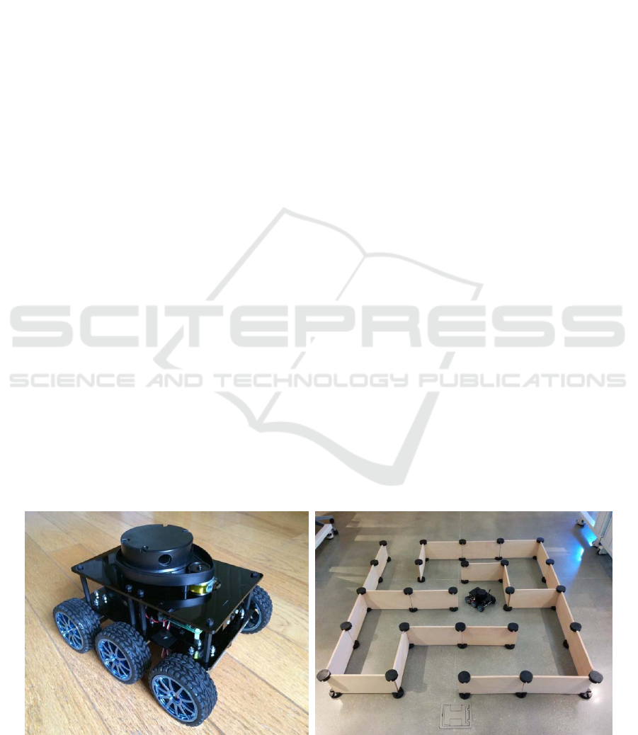
The ciNeuroBot (Figure 1) has been designed to
simulate and explore goal-oriented behaviors
exhibited by rats running in mazes (Bieszczad, 2006).
The robot’s name is derived from the Neurosolver, a
neuromorphic high-level planner based on the
organization of columns in the brain cortex
(Bieszczad, 1998).
The ciNeuroBot is based on the DiddyBorg
platform integrated with a 360-degree LIDAR planar
scanner placed at the top. The robot has six wheels
powered by six engines that are controlled in two
groups: left and right. The hardware controller
utilizes RaspberryPI single-board-computer running
Raspbian version of Linux. There is also a high-
resolution video camera in front of the robot, but it is
not used for navigation. The code is written in Python
3 taking advantage of generous supply of modules
and a relatively high computational power of the
platform.
Figure 1: ciNeuroBot and ciNeuroBot in a reconfigurable maze.
Bieszczad, A.
Using Inverse Compensation Vectors for Autonomous Maze Exploration.
DOI: 10.5220/0006437203970404
In Proceedings of the 14th International Conference on Informatics in Control, Automation and Robotics (ICINCO 2017) - Volume 2, pages 397-404
ISBN: Not Available
Copyright © 2017 by SCITEPRESS – Science and Technology Publications, Lda. All rights reserved
397
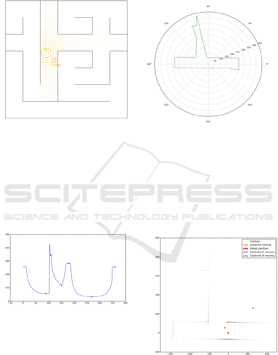
Figure 2: ciNeuroBot simulator with a LIDAR simulated
scan of the right t-section cue.
The ultimate high-level task of the robot is to
explore mazes like the one shown in Figure 1
searching for goals; for example, certain colors or
shapes on the walls (the video camera is used for that
purpose). Furthermore, the robot is to construct a map
of the maze and record the location of the goals, so in
the future it can construct a plan recalling – and
potentially optimizing – the paths to a specific goal.
The construction of the map is founded on the ability
to identify environmental cues; in the case of a maze,
the cues are perceived shapes such as cross-section, t-
section, right turn, left turn, etc.
Figure 3: LIDAR scan of the right t-section cue. The scan
readings (on the vertical axis) are shown as a function of an
angle from which the measurement was made. There are
360 measurements for a full rotation of the scanner. Also,
the minima on the curve are shown as red dots (the
rightmost minimum is there due to a cyclic wrap of the
curve). The scan starts from the back of the robot and
proceeds counter clockwise.
To realize the high-level objectives, the robot
needs low-level capabilities to autonomously explore
the maze staying clear of walls.
Figure 4: LIDAR scan readings of right t-section cue shown
in polar coordinates. The orientation is different than in
Figure 2 due to the 90-degree rotation. The robot is always
in the center of any coordinate system; in this case, polar.
We developed a simulator of the robot running
mazes (Figure 2) to ease – and in some cases, make
feasible – the experimentation and development. The
simulator is tightly correlated with the physical robot,
so the ideas implemented and tested in the simulator
can be used to create prototypes to be transferred to
the physical robot. As we found out however, the
physical world poses challenges that need attention
during the porting such as imperfections in the
accuracy of scanner readings.
Figure 5: Maze contour constructed from the LIDAR
readings of right t-section cue. The red dot demarcates the
position of the robot. The dot is also in the center of the
Cartesian coordinate system.
ICINCO 2017 - 14th International Conference on Informatics in Control, Automation and Robotics
398

The onboard LIDAR scanner is used for both the
high- and the low-level functionality. At the high-
level, the mapping and localization components need
cues that can be identified using the LIDAR readings
(Figure 3) (Bieszczad, 2015 and the ongoing research
on improving that capability).
The LIDAR readings (that are simply the
distances from the objects in the robot surroundings;
i.e., walls in a maze in this case) can also be used to
keep the robot away from the walls. The robot moves
are controlled by a velocity vector generated in
response to some mobility drive that may be coming
from a manual robot controller (e.g., our Android or
iOS apps), or from a higher-level planner like the
Neurosolver. To keep the robot away from the walls,
the velocity vector must be modified by analyzing the
LIDAR readings. The periodic compensation allows
the robot to stay within the walls while moving along
the modified velocity vector.
2 OBSTACLE AVOIDANCE
PROBLEM
The problem of avoiding obstacles is one of the most
critical in Robotics. A very good survey of the
approaches, especially techniques based on
commonly used potential fields is presented in
(Rajvanshi et al., 2015). The methods based on
potential fields (originally proposed in (Khatib,
1986)) assume presence of a target destination that
acts as an attractor force for the robot, while any
surrounding obstacles act as repellent forces. The
problem of exploring a maze is somewhat different,
as the obstacles are the enclosing walls, and there is
no global target. Rather than being repelled to some
open space by the obstacles, robot’s objective is to
stay within the maze walls in a position equidistant
from any wall while still maintaining the movement.
The overall problem can be summarized as a task
of moving as far as possible from each of the
obstacles at every step in the movement. While
conceptually the task is simple, it is an optimization
problem, and as such, it is computationally
demanding. The problem is especially challenging for
robots that have limited processing power and limited
information about the environment; for example, if
the robot – like ciNeuroBot – is equipped with just a
simple one-dimensional scanner (also referred to as
planar or 2D scanner). Simple methods – like
computing a centroid of certain “important” set of
points on the obstacles – fail in complex scenarios.
For example, if the robot is close to several obstacles
that are also close to each other, it will tend to move
towards the obstacles if the centroid is used as a
guidance. In a maze, quite often the centroid is
completely inaccessible; as exemplified by the point
marked with blue cross in Figure 5. A centroid of the
closest points – shown as a green triangle in the same
figure – might be better, but still fails in numerous
scenarios. Our experiments with computing a
centroid of the convex hull spanned by the closest
points from the robot to the walls also led to only
marginal improvements.
It appears that there is no known closed form
solution to the problem. While iterative solutions do
exist, they are computationally expensive (Eppstein,
Erickson, 1999). Most of the solutions that have been
proposed approximate the “center of view” (the point
as distant from each of the obstacles as possible;
sometimes also called the “center of gravity”) by
iteratively decomposing the map using triangles
(Shewchuk, 2008), or quad-trees (Agafonkin, 2016;
based on Finkel, 1974). The medial axis transform
(MTA) has also been used (Joan-Arinyo et al., 1997
based on Lee, 1982). Like the potential fields
methods, the MTA is used usually in context of path
planning; some researchers advocate separation of
path planning from the obstacle avoidance problem
and treating them as two distinct issues. Point
sampling was also attempted to approximate the
location that is optimally furthest from all obstacles
(Garcia-Castellanos, Lombardo, 2007).
An obstacle avoidance strategy based on direction
correction based on the distances from obstacles (that
could be viewed as a density of obstacles) was
reported in (Peng et al., 2015) as part of path planning
research.
3 INVERSE COMPENSATION
VECTOR (ICV)
We propose a simple and efficient way to compensate
the robot movement by computing a correction vector
that we call the Inverse Compensation Vector, or
ICV. As stated earlier, the direction and the speed of
a moving robot can be expressed as a velocity vector
(or force). It is the velocity vector that is affected by
applying the Inverse Compensation Vector to correct
the movement with the intention of staying away
from the walls. Ultimately, that motion compensation
operation implements a simple collision avoidance
algorithm.
In the following sections, we focus on the
construction of the ICV; the velocity vector is not
Using Inverse Compensation Vectors for Autonomous Maze Exploration
399
included in the figures as it may be arbitrarily
imposed at any time.
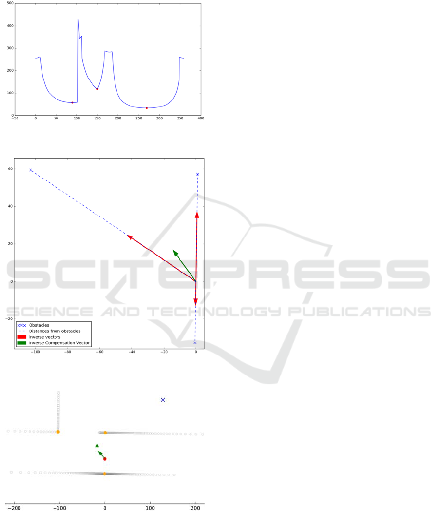
Figure 6: LIDAR scan readings for right t-section cue with
the three smallest minima shown as red dots.
Figure 7: Graphical illustration of constructing the Inverse
Compensation Vector (ICV) for the right t-section cue.
Figure 8: The ICV for the right t-section cue versus the
centroid of the contour and the centroid of the supporting
contour (see the text for explanation).
The ICV is constructed on the basis that the robot
should be kept away from each of the points in a
contour of the maze as far as possible. In contrast to
the potential fields approach, obstacles are seen as
attractors rather than repellents. Rather than pushing
the robot away, they pull it to a position in which all
forces are balanced. As stated earlier, finding such a
center of gravity is an optimization problem that is
computationally hard. However, the following
approach yields reasonable computational results in
simulations.
The algorithm assumes that the robot position is
always in the center of the coordinate system. We
compute a set of minima in the LIDAR scan reading
shown as red dots in Figure 3. Next, we select three
closest points in the contour (i.e., the smallest
minima). Figure 6 shows the same scan as in Figure
3, but with only three smallest minima. We already
discussed constructing a contour of the maze from the
LIDAR readings; an example is shown Figure 5.
Using the minima, we can select the closest contour
points for any set of minima; we call the set a
supporting contour. The points in two-dimensional
space correspond to vectors (with the center of the
coordinate system as the other end), so we call the
closest three contour points support vectors. Support
vectors are the basis for computing the ICV. To do
that, a mean distance to all points in the supporting
contour is computed. Then we calculate inverse ratios
of the mean to the support vectors; the smaller the
vector, the larger the ratio. The adjective inverse
refers to the fact that instead of normalizing the
vectors using their mean, inverses of these
normalizations are computed. The ratios are then used
to compute inverse vectors that attract the robot
towards the gaps between the robot and each of the
points in the supporting contour. The idea follows the
logic that the robot should move into empty spaces
between itself and the obstacles with the speed
inversely related to its distance to a given obstacle.
The further the obstacle (i.e., the larger the gap) the
more attractive it is to move towards the that obstacle
(relatively to the other obstacles). Hence, using the
metaphor from the potential field methods, the
obstacles attract the robot with a force relative to the
inversely normalized distance from the robot. We
refer to the operation as inverse compensation.
A Python 3 snippet to compute the ICV is shown
in Code Snippet 1. In the code, the support vectors are
passed as a parameter vs. In addition to the ICV, the
function also returns the compensation vectors as well
as their mean. The additional return values could be
used for scaling the ICV in some circumstances; for
example, in relation to the width of the maze
passages.
ICINCO 2017 - 14th International Conference on Informatics in Control, Automation and Robotics
400

Code Snippet 1: Python 3 code to compute the Inverse Compensation Vector icv of three vectors given as a Numpy array vs.
Figure 7 illustrates the process using a scan of the
right t-section cue as an example. The robot position
is in the center of the coordinate system (the base of
all shown vectors). The crosses demarcate the closest
obstacles with broken lines reflecting the distances.
The red vectors are the individual inverse
compensation vectors, and the green arrow is the total
inverse compensation vector (i.e., the mean of the
individual inverse vectors). That is the vector that
would be used to compensate the motion drive vector
of the robot.
The result of the computation in the context of the
contour, the centroid of all contour points, as well as
the centroid of the supporting contour is shown in
Figure 8. The difference with the centroid of all points
is dramatic, but not so much with the centroid of the
supporting contour. As shown in the following
experiments the difference may be much more
significant in other cases.
4 RESULTS
Currently, we have defined six cues in the maze: right
turn, left turn, t-section, cross-section, right t-section,
and left t-section. Figure 9 shows calculations of the
ICVs for arbitrary robot positions in approaching
each of the cues.
It is evident from the illustrations that ICVs
(shown as green arrows) provide much improved
correction to robot movement over using a centroid
of the supporting contour (shown as a green triangle).
While the centroid point often lays even closer to the
obstacles than the current robot position, the ICVs
direct the robot to much safer locations. It is worth
noting that using potential fields methods would
direct the robot away from all points on the
supporting contour and as such would not be suitable
for this application.
To gain some insight into the movement
compensation calculations for different robot
positions near a single cue, we conducted a series of
experiments in which we calculated ICVs for
different robot locations when near a selected cue.
Figure 10 illustrates how the ICV evolves with the
change of the robot position when approaching the t-
section cue (that we used earlier in this document to
demonstrate the process of constructing the ICV). We
can see that every correction to the position is very
reasonable and balances the overall distance from all
the obstacles. Experiments with other cues and other
locations also support that thesis.
import numpy as np
def compute_icv(vs):
# compute vector lengths
vs_len = np.sqrt((vs*vs).sum(axis=1))
# get a mean length
vs_mean_norm = np.mean(vs_len)
# compute inverse proportions
inv_factor = vs_mean_norm/vs_len
# calculate correction vectors by applying inverse
# proportions to the vectors
vs_inv_norm = vs - np.array([k * v for k,v in zip(inv_factor, vs)])
# compute the final correction vector as the mean
# of correction vectors
icv = vs_inv_norm.mean(axis=0)
return icv, vs_inv_norm, vs_mean_norm
# Example
vs = np.array([[ 23, -18],
[ -7, -24],
[ 19, 23],
[-14, 2],
[-24, -3]])
compute_icv(vs)
Using Inverse Compensation Vectors for Autonomous Maze Exploration
401
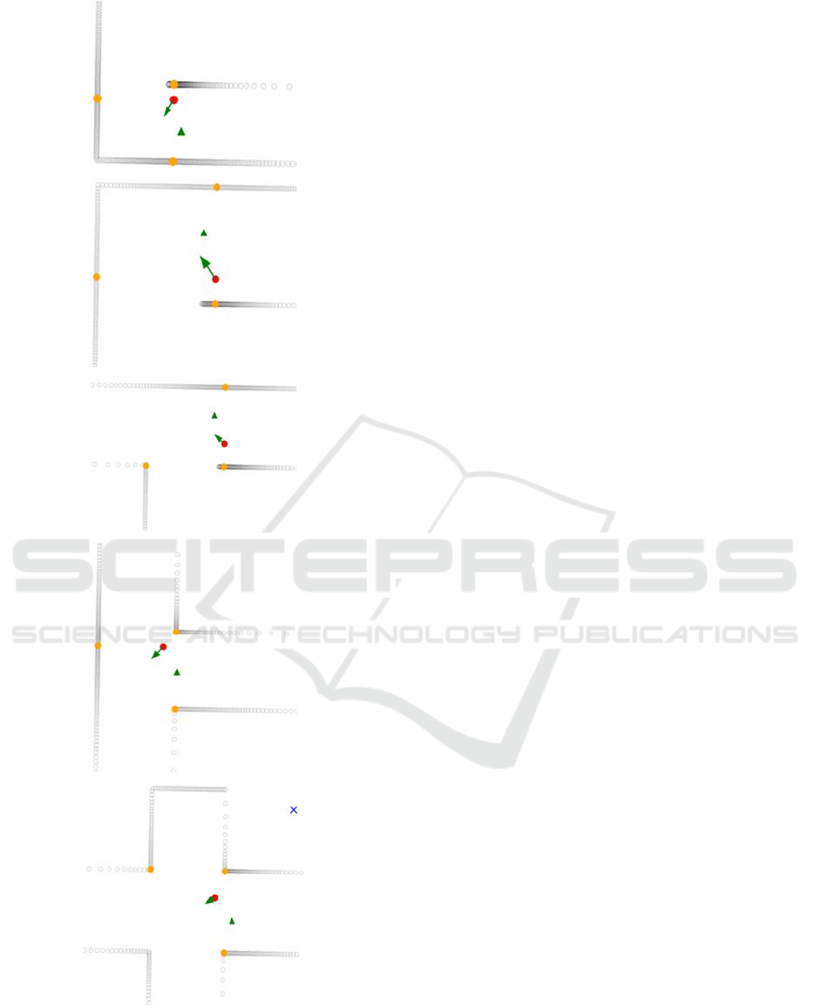
Figure 9: The ICVs (green arrows) for (from top to bottom):
right turn, left turn, left t-section, t-section, and cross-
section. The ICV for right t-section is shown in Figure 5.
5 HEURISTICS
5.1 Noisy Data
The LIDAR data collected in the simulator are perfect
as they are computed using Mathematically sound
formulas. However, the data that are collected from a
LIDAR residing on a physical robot placed in an
actual maze contain noise that constitutes a challenge
for a reliable identification of minima. Very often the
measured distances that are angularly close to each
other differ by small amounts due to the imperfect
accuracy of the LIDAR. That yields distance curves
that are rugged, and as such prone to containing
numerous local minima as shown in the upper plot of
Figure 11 as tightly located red dots (they look almost
as thick red lines).
To deal with that problem, we applied a
smoothing function that removes the excess of local
minima as shown in the lower plot in Figure 11.
5.2 Tight Support Contours
If the distance minima are close to each other both by
angle and by magnitude, the ICV may not have the
magnitude sufficient to repel the robot from the walls.
There are two ways of dealing with the problem. First
is to ensure that the minima are well distributed in the
span of the scan. Therefore, the LIDAR full 360
degrees range is divided in several equal zones, and
then minima are calculated for each of the zones. The
three smallest are then used in computing the ICV.
The minima shown in the lower plot of Figure 11
were obtained in the described way.
Another method that we tried was to use an
inverse of the variance in the distances to the
obstacles to modulate the magnitude of inverse
vectors. That method helped only in some cases; for
example, when the robot was close to three obstacles
located closely one to another. Applying zoning to
finding minima make such scenarios impossible, so
this approach was abandoned.
6 CONCLUSIONS
Our simulations show that correcting the robot
velocity vector by the Inverse Compensation Vector
(ICV) is a very simple yet effective approach to
keeping the robot away from the maze walls. The ICV
that corrects both the direction and the speed is
computed and applied periodically after each of the
ICINCO 2017 - 14th International Conference on Informatics in Control, Automation and Robotics
402
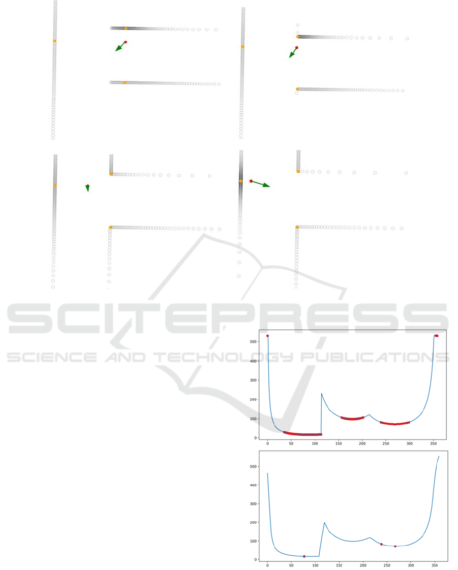
Figure 10: The ICVs computed for four different location of the robot near a t-section cue.
LIDAR scans (or as often as the processing power of
the robot controller allows).
The method does not yield an optimal solution to
the obstacle avoidance problem, but is much more
efficient than the iterative approaches to finding the
center of gravity discussed in the introduction.
Therefore, it can be applied in robots that employ
relatively slow processor boards.
7 FUTURE WORK
We are transferring the algorithms to the physical
robot. The simulator does not take into account the
volume of the robot, so some adjustments are
necessary to the use of the ICV.
We are also looking at the scaling of the speed
correction, since certain scenarios may yield ICVs
that, for example, just cancel out the motion drive
vector leading to halting the robot altogether. This is
not a problem with a remote controller as just more
forward movement might be applied. However, an
autonomous robot must have a logic to deal with such
issues. We theorize that a detection of a stop can be
used to modify the velocity vector. A stop detector is
easy to implement by comparing subsequent LIDAR
scans.
Figure 11: Cleaning up the noise data using smoothing and
ensuring distribution using zones. The upper plot shows
raw data, and the bottom shows the distance curve after it
was smoothened and divided in three sectors.
Using Inverse Compensation Vectors for Autonomous Maze Exploration
403

The further-reaching agenda includes the goal-
oriented behavior that we described in the
introduction. We are making progress using the
simulator, but to transfer the ideas to the physical
robot we must tackle other low-level tasks similar to
the ones described in this report.
ACKNOWLEDGEMENTS
The author would like to acknowledge assistance
from two research assistants and excellent senior
Computer Science students Jesus Bamford and Corey
Smith, who are implementing many of the ideas and
conduct a lot of tests, especially with the physical
robot. This work would not be possible without them.
Great thanks to both!
REFERENCES
Agafonkin, V., 2016 (snapshot). A new algorithm for
finding a visual center of a polygon.
https://www.mapbox.com/blog/polygon-center/.
Aichholzer, O., Aurenhammer, F., Alberts, D., and Gartner,
B., 1995. A novel type of skeleton for polygons. In
Journal of Universal Computer Science 1(12):752-761,
1995.
Bieszczad, A. and Pagurek, B., 1998. Neurosolver:
Neuromorphic General Problem Solver. In Information
Sciences: An International Journal 105 (1998), pp.
239-277, Elsevier North-Holland, New York, NY.
Bieszczad, A. and Bieszczad, K., 2006. Running Rats with
Neurosolver-based Brains in Mazes. In Proceedings of
International Conference on Artificial Intelligence and
Soft Computing, Zakopane, Poland.
Bieszczad, A., 2015. Exploring Machine Learning
Techniques for Identification of Cues for Robot
Navigation with a LIDAR Scanner. In Proceedings of
12th International Conference on Informatics in
Control, Automation and Robotics (ICINCO 2015),
Special Session on Artificial Neural Networks and
Intelligent Information Processing (ANNIIP 2015),
Cormal, France, CITEPRESS Digital Library.
DiddyBorg, 2017 (snapshot).
https://www.piborg.org/diddyborg
Eppstein, D., Erickson, J., 1999. Raising roofs, crashing
cycles, and playing pool: Applications of a data
structure for finding pairwise interactions. In Discrete
& Computational Geometry 22(4):569-592.
Finkel, R., Bentley, J.L., 1974. Quad Trees: A Data
Structure for Retrieval on Composite Keys. In Acta
Informatica 4 (1): 1–9.
Garcia-Castellanos, D., Lombardo, U., 2007. Poles of
Inaccessibility: A Calculation Algorithm for the
Remotest Places on Earth. In Scottish Geographical
Journal Vol. 123, No. 3, 227 – 233.
Joan-Arinyo, R., Pérez-Vidat, L., Gargallo-Monllau, E.,
1997. An Adaptive Algorithm to Compute the Medial
Axis Transform of 2-D Polygonal Domains. In
Proceeding CAD Systems Development: Tools and
Methods Pages 283-298, Springer-Verlag London, UK.
Khatib, O., 1986. Real-time obstacle avoidance for
manipulators and mobile robots. In International
Journal of Robotics Research, Volume 5 Issue 1, pp.
90-98, SAGE Publications.
Lee, D. T., 1982. Medial Axis Transformation of a Planar
Shape. In IEEE Transactions on Pattern Analysis and
Machine Intelligence Volume: PAMI-4, Issue: 4.
Peng, Y., Qu, D., Zhong, ,Y., Xie, S., Luo, J., Gu, J., 2015.
The Obstacle Detection and Obstacle Avoidance
Algorithm Based on 2-D Lidar. In Proceeding of the
2015 IEEE International Conference on Information
and Automation Lijiang, China.
Rajvanshi, A., Islam, S., Majid, H., Atawi, I., Biglerbegian,
M., and Mahmud, S., 2015. An Efficient Potential-
Function Based Path-Planning Algorithm for Mobile
Robots in Dynamic Environments with Moving Targets.
In British Journal of Applied Science & Technology
9(6): 534-550.
RPLIDAR, 2017 (snapshot).
https://www.seeedstudio.com/RPLIDAR-360-degree-
Laser-Scanner-Development-Kit-p-1823.html
Shewchuk, J. R., 2008. "General-Dimensional Constrained
Delaunay and Constrained Regular Triangulations, I:
Combinatorial Properties". 39 (1-3): 580–637.
Yan Peng, Y., Dong Qu, D., Yuxuan Zhong, ,Y., Shaorong
Xie, S., Jun Luo, J., Jason Gu, J., 2015. The Obstacle
Detection and Obstacle Avoidance Algorithm Based on
2-D Lidar. In Proceeding of the 2015 IEEE
International Conference on Information and
Automation Lijiang, China.
ICINCO 2017 - 14th International Conference on Informatics in Control, Automation and Robotics
404
