Design and Stiffness Analysis of 12 DoF Poppy-inspired Humanoid

Dmitry Popov, Alexandr Klimchik and Ilya Afanasyev

Institute of Robotics, Innopolis University, Universitetskaya Str. 1, Innopolis, Russia

Keywords:

Stiffness Modeling, Human Mechatronics, Motion Control Systems, Robot Kinematics.

Abstract:

This paper presents a low-cost anthropomorphic robot, considering its design, simulation, manufacturing and

experiments. The robot design was inspired by open source Poppy Humanoid project and enhanced up to

12 DoF lower limb structure, providing additional capability to develop more natural, fast and stable biped

robot walking. The current robot design has a non-spherical hip joint, that does not allow to use an analytical

solution for the inverse kinematics, therefore another hybrid solution was presented. Problem of robot joint’s

compliance was addressed using virtual joint method for stiffness modeling with further compensation of elas-

tic deﬂections caused by the robot links weight. Finally, we modeled robot’s lower-part in V-REP simulator,

manufactured its prototype using 3D printing technology, and implemented ZMP preview control, providing

experiments with demonstration of stable biped locomotion.

1 INTRODUCTION

The progress in creation of highly specialized robotic

systems contributes to automation of different every-

day life aspects that can partially or fully replace hu-

mans in the future in some routine activities. The

development of androids is one of the most relevant

solution for successful robot operations in human en-

vironment with enhanced functionality. These robots

usually resemble human beings in appearance and/or

internal construction, having the similar body shape

structure and walking principles. One of the most im-

portant part of an anthropomorphic robot is a pelvis

with the lower limbs, which form the lower-part body.

During last decades, robotics community has pro-

posed some successful models of biped robots with

similar lower limb structure with 6 Degree of Free-

dom (DoF) per leg, having 3 DoF hip, 1 DoF knee,

and 2 DoF ankle. Thus, there are some well-known

human-size androids like Honda ASIMO (Sakagami

et al., 2002), WABIAN from Waseda University (Ya-

maguchi et al., 1999), Boston Dynamics Atlas (not a

commercially available model), Pal Robotics Reem-

C (Ferro and Marchionni, 2014), Android Technics

AR-600 (Khusainov et al., 2015), etc. But for small-

size robots the most popular models are ROBOTIS

Darwin (Ha et al., 2011), Aldebaran Robotics Nao

(Gouaillier et al., 2009) and Poppy Humanoid

with

Open source Poppy Humanoid project, www.poppy-

project.org

5 DoF leg (Lapeyre et al., 2013b).

Stiffness modeling in robotics is considered for in-

dustrial manipulators, where problem of end-effector

precise positioning under external and internal load

are critical (Pashkevich et al., 2011). In humanoid

robots accurate positioning is not always necessary,

but with high compliance in links or joints, deﬂections

caused by payload or link weights can affect robot sta-

bility. Therefore those deﬂections should be consid-

ered and compensated as possible.

Our goals in this paper are:

1. Adapt Poppy-like robot to new mechanical struc-

ture with 6 DoF lower limbs, which are able

to support robot’s upper-part (including a torso,

hands, a head, sensors and a possible payload).

2. Implement stiffness model of the robot.

3. Develop software for fast, stable robot walking

that also considers robot joints compliances and

successfully eliminates them.

4. Reduce the robot production cost using hobby ser-

vomotors, inexpensive fabrication methods and

cost-efﬁcient electronics components.

The rest of the paper is organized as follows. Sec-

tion 2 presents the robot design. Section 3 consid-

ers robot lower body’s kinematics analysis includ-

ing forward, inverse kinematic problem and robot

workspace. Section 4 describes stiffness model. Sec-

tion 5 includes trajectory planning and compensation.

Popov, D., Klimchik, A. and Afanasyev, I.

Design and Stiffness Analysis of 12 DoF Poppy-inspired Humanoid.

DOI: 10.5220/0006432000660078

In Proceedings of the 14th International Conference on Informatics in Control, Automation and Robotics (ICINCO 2017) - Volume 2, pages 66-78

ISBN: Not Available

Finally, we conclude in section 6 with discussion on

future work.

2 ROBOT DESIGN

The main feature of two-legged robot platform is the

ability to walk. Therefore, the human body has been

taken as a reference of the most advanced two-legged

mechanism. In general human leg has dozen of DoF,

but in case of bipedal walking, leg motions can be ap-

proximated with 6 DoF, three in the sagittal plane (an-

kle, knee, hip), one in the horizontal plane (hip) and

two in the frontal plane (hip, ankle). Existing open

source project Poppy has only 5 DoF per leg, 3 DoF

in hip, 1 DoF in knee, and 1 DoF in ankle. In order

to use standard 6 DoF approximation, addition DoF

was added in the ankle. Usage of expensive Robo-

tis Dynamixel MX-28, MX-64 is another problem of

Poppy. To reduce overall cost of the robot, we pro-

pose to use more cheaper SpringRC SR-518 servo-

motors with 2 Nm torque and RS485 bus connection.

Mounting places were also altered in order to ﬁt this

new motors.

Since human thigh bones are inclined by 6-7 de-

grees, it was also implemented by (Lapeyre et al.,

2013a) in Poppy robot and our robot limb design. It

allows to reduce falling speed and decrease the lateral

motion of torso for single support phase and double

support phase respectively. In order to make robot

construction lighter and stiffer, we used mesh struc-

ture for thigh and shin.

Usually, most biped robots have unproportionally

big foot. It is required in order to increase pas-

sive stability with increased support polygon. In our

project, the foot size is proportional to human foot,

thus providing additional difﬁculties to stabilization

algorithms, but at the same time increasing robot mo-

bility (Lapeyre et al., 2014).

(a) 3D printed prototype. (b) Model in V-REP.

Figure 1: Bipedal robot.

Table 1: Robot model joint range of motion.

Joint

Human (deg.) Robot (deg.)

Hip Y

-30 to 45 -25 to 45

Hip Z

-45 to 50 -40 to 60

Hip X

-15 to 130 -60 to 100

Knee X

-10 to 155 -6 to 112

Ankle X

-20 to 50 -35 to 30

Ankle Y

-30 to 60 -35 to 35

Table 2: Robot model mass parameters.

Name Mass (kg) Mass Poppy (kg)

Thigh 0.226 0.239

Shin 0.124 0.108

Foot 0.116 0.047

Total 1.21 1.14

Table 3: Robot model size parameters.

Name Size (mm) Size Poppy (mm)

Thigh 181 181

Shin 178 177

Foot 129 x 63 145 x 50

Total 129 x 200 x 500 145 x 187 x 495

According to Table 1, robot leg’s motion range is

close to human, excepting joints with rotation around

X axis. Their range is enough for walking, but can

limit robot maneuverability for other activities. The

limitations on joint motion range will be considered

in Section 5.

In order to specify requirements to the robot

hardware part, the combination of Dassault Systmes

SolidWorks CAD tool and robot simulator Coppelia

Robotics V-REP were used (Rohmer et al., 2013).

Robot prototype was manufactured using Fused

Deposition Modeling (FDM) technique with Acry-

lonitrile butadiene styrene (ABS) polymer. It allows

to reproduce robot mechanical part on every low-cost

3D printer.

Manufactured prototype and robot model in sim-

ulation environment are shown in Figure 1a and 1b

correspondingly. Table 2 and 3 shows proposed robot

mass and size parameters in comparison with lower

half of Poppy robot. Total mass and size parame-

ters remains the same, despite additional servomotor

in ankle joint (6th DoF).

Design and Stiffness Analysis of 12 DoF Poppy-inspired Humanoid

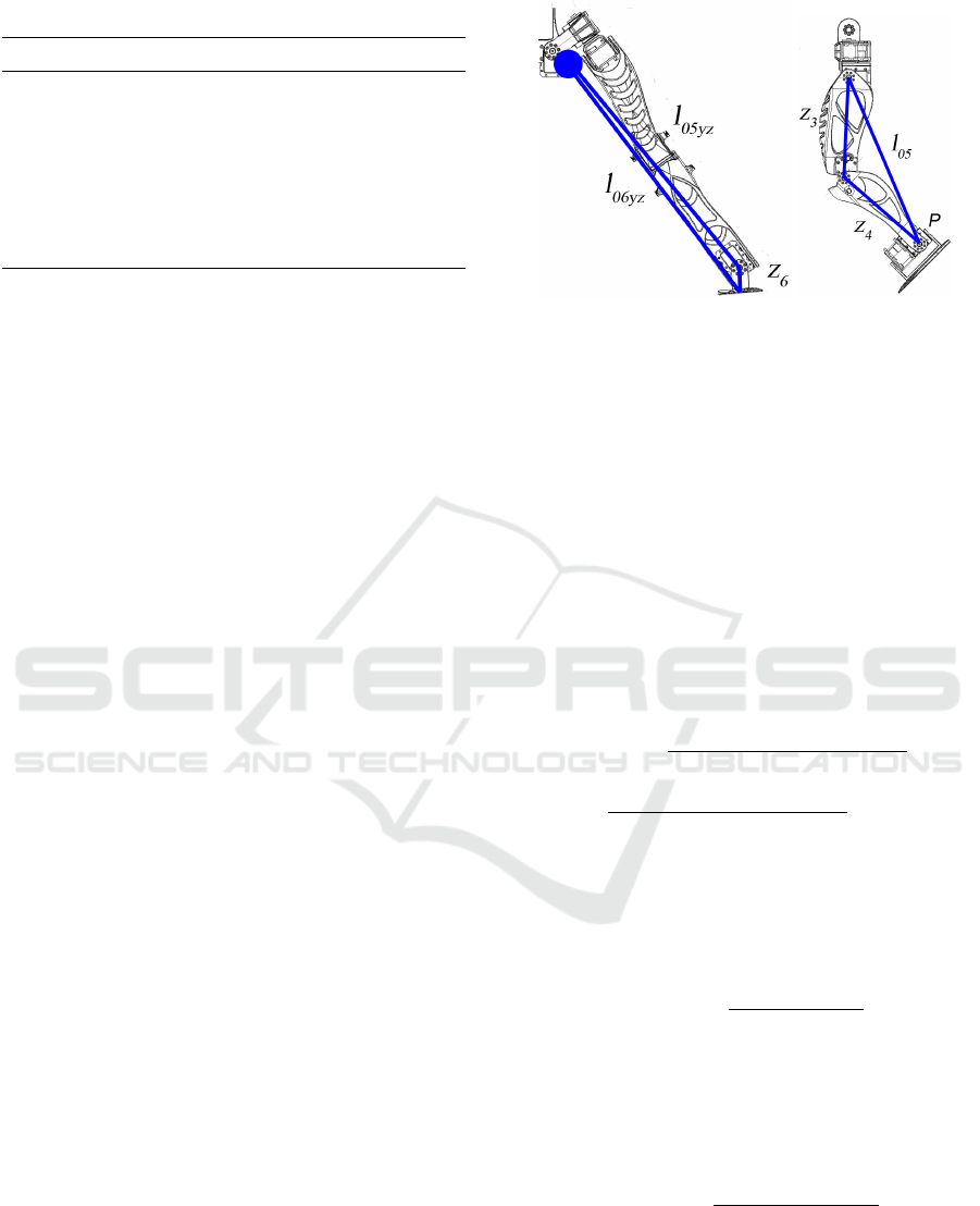
Table 4: Robot model mDH parameters.

, mm a

n−1

, mm α

n−1

, rad Offset

q1 0 19 (y0) π/2 0

q2 47 (z2) 52 (y1) π/2 π/2

q3 0 0 π/2 π/2

q4 -23 (-y3) 181 (z3) 0 0

q5 0 178 (z4) 0 0

q6 0 0 π/2 0

3 KINEMATICS MODELING

3.1 Forward Kinematics

Forward or direct kinematics is the task of determin-

ing the position and orientation of the end-effector by

giving conﬁguration of the robot. The robot can be

modeled as a kinematic chain of 7 links connected

by 6 joints. The base frame of the robot located in

the center of the waist. The local frames are assigned

to joints, according to modiﬁed Denavit-Hartenberg

(mDH) convention presented in (Craig, 2005). Ta-

ble 4 shows robot mDH parameters. Since the right

and left leg are identical, kinematics only for one leg

will be considered.

T F = T 0 ∗T1 ∗ T 2 ∗ T 3 ∗ T 4 ∗ T 5 ∗ T 6 ∗ T 7 =







r11 r12 r13 T x

r21 r22 r23 Ty

r31 r32 r33 T z

0 0 0 1







(1)

Final transformation matrix T F from the base to the

end-effector can be obtained by multiplying transfor-

mational matrices of all joints (1).

3.2 Inverse Kinematics Problem

The purpose of solving the inverse kinematics (IK) is

to ﬁnd the angle of each joint for a known foot posi-

tion and orientation. IK can be solved in two different

ways: analytically and numerically. Analytical solu-

tion for 6 DoF serial manipulator can be hard to obtain

directly or geometrically like in chapter 1 (Siciliano

and Khatib, 2008), so different advanced techniques

like Pieper method are usually used.

3.2.1 Analytical Solution

For solving IK with (Peiper, 1968) method serial ma-

nipulator should have 3 joints with consecutive axes

(a) Frontal plane. (b) Sagittal plane.

Figure 2: Robot leg.

intersecting at one point. Its not possible to use it for

the considered robot. Therefore, let us consider an-

other, similar modiﬁcation, with spherical joint in the

hip.

In order to simplify inverse kinematics, it is pos-

sible to ﬁnd a geometrical solution for frontal (Fig-

ure 2a) and sagittal (Figure 2b) planes separately. In-

termediate steps of ﬁnding inverse kinematics solu-

tion can be found in appendix of this paper.

q1 = sin

−1

(r32 · cos(q6) − r33 · sin(q6)) (2)

q2 = atan2



r12 · cos(q6) − r13 · sin(q6)

−cos (q1)

r22 · cos(q6) − r23 · sin(q6)

cos(q1)



(3)

q3 = atan2(−z4 · sin(q4) · A+

(z3 + z4 · cos(q4)) · B,

z4 · sin(q4) · B + (z3 + z4 · cos(q4)) · A)

(4)

q4 = cos

−1



− z3

− z4

2 · z3 · z4



(5)

q5 = atan2 (−r11 · sin(q1)sin (q2)+

r21 · cos(q2)sin (q1) −r31 · cos(q1),

r11 · cos(q2) + r21 · sin (q2)) −q3 − q4

(6)

q6 = cos

−1

06yz

− l

05yz

− z6

2·l

05yz

· z6

(7)

Equations (2-7) shows solutions for inverse kinemat-

ics problem for 6 DoF robot with spherical hip.

ICINCO 2017 - 14th International Conference on Informatics in Control, Automation and Robotics

3.2.2 Numerical Solution

The inverse kinematics problem in the general case

is the searching for the solution of a set of nonlin-

ear algebraic equations. Most popular methods are

the iterative ones. The most common method is the

Newton-Raphson method, that can be found in (Jazar,

2010).

Before solving inverse kinematics with numerical

method it necessary to ﬁnd Jacobian of the robot.

The time derivative of the kinematics equations

yields the robot Jacobian, which deﬁnes the joint con-

tribution to the linear and angular velocity of the end-

effector. Jacobian matrix has the size of 6xN, where

N number of DoF. It consists of two parts: Transla-

tional and Rotational. Jacobian for left leg:

(q) =



(q)



(8)

where J

(q) – translational part; J

(q) – rotational

part.

Jacobian can be computed as the time derivative

of forward kinematics equations, with skew theory,

or as numerical derivatives. In this work, numerical

derivatives were used.

T F = T 0 ∗ [T (k − 1)(q,π) ∗ H(π

)∗

T (k + 1)(q,π)] ∗ T 7

(9)

= T 0 ∗ [T (k − 1)(q,π) ∗ H

(π

)∗

T (k + 1)(q,π)] ∗ T 7

(10)

where T (q,π) - the transformation matrices on the left

and right sides of the currently considered parameter

, H

(π

) is the differential transformation matrix.

Elements of Jacobian will be equal to:

π,k







k, (1,4)

k, (2,4)

k, (3,4)

∗ T F

−1

]

(3,2)

∗ T F

−1

]

(1,3)

∗ T F

−1

]

(2,1)







(11)

There are numerous ways how to use Jacobian,

but one of the most popular ones are pseudoinverse

method and damped least square (DLS) method. The

pseudoinverse method is widely discussed in the lit-

erature, but it often performs poorly because of in-

stability near singularities. The damped least square

method has better performance (Buss, 2004). Both of

these methods were implemented and compared.

3.2.3 Hybrid Solution

In the proposed robot conﬁguration hip joint is not

spherical since the ﬁrst three axes do not intersect at

one point that means that previously described analyt-

ical solution cannot be used. Thus, numerical solution

in this case shows non constant efﬁciency.

In order to improve numerical method efﬁciency

a hybrid approach from (Cisneros Lim

on et al., 2013)

is used. It consists of two phases. Phase one is

to obtain approximate solution, since similar robot

conﬁguration with spherical hip joint is very close

to our robot conﬁguration. Phase two – use this

approximate solution as initial for numerical method.

It allows to greatly reduce the number of iterations.

The hybrid algorithm of inverse kinematics:

1. Set the initial counter i = 0.

2. Find q(0) by using analytical solution of similar

robot.

3. Calculate the residue δT (q(i)) = J(q(i))δq(i). If

every element of T (q(i)) or its norm ||T (q(i))|| is

less than a tolerance, ||T (q(i))|| < ε then termi-

nate the iteration. The q(i) is the desired solution.

4. Calculate q(i + 1) with pseudoinverse or DLS or

any other technique.

5. Set i = i + 1 and return to step 3.

The performance of the hybrid and numerical al-

gorithm was compared in order to evaluate its efﬁ-

ciency. The main evaluation parameters are (1) the

number of iterations, which is needed to ﬁnd a de-

sired precision and orientation, and (2) the mean time

required for computing this solution.

This evaluation was carried out over a data set

consisting of 750 points along gait trajectory. Desired

accuracy for numerical algorithm is equal to 10

−6

Desired end effector position in X, Y, Z coordinates

is shown in Figure 9a - 9c, whereas achieved joint

angles is shown in Figure 9d. The results of the eval-

uation are shown in Table 5.

Table 5: Performance comparison of inverse kinematics al-

gorithms.

Indicator

Iterations,

Execution

time, ms

Analytical 1 0.04

Hybrid DLS 4 0.24

Numerical

DLS

104 4.46

Numerical

pseudoinverse

205 14.24

Design and Stiffness Analysis of 12 DoF Poppy-inspired Humanoid

Hybrid solution is up to 20x faster than numeri-

cal DLS. It also has 100% cover rate, which means

that all points of the test set (inside workspace) were

reached. This algorithm allows real-time calculation

with 50 Hz control loop, which is maximum for used

robot.

3.3 Workspace Analysis

The workspace of a manipulator is deﬁned as the vol-

ume of space, which the end-effector can reach. Two

different deﬁnitions of workspace are usually used. A

reachable workspace is the volume of space within

which every point can be reached by the end effec-

tor in at least one orientation. A dexterous workspace

is the volume of space within which every point can

be reached by the end effector in all possible orienta-

tions. The dexterous workspace is a subset of reach-

able workspace (Jazar, 2010; Siciliano and Khatib,

2008).

According to robot task - forward walking on the

ﬂat surface, only inclusive orientation workspace is

needed. In this case end-effector orientation locked

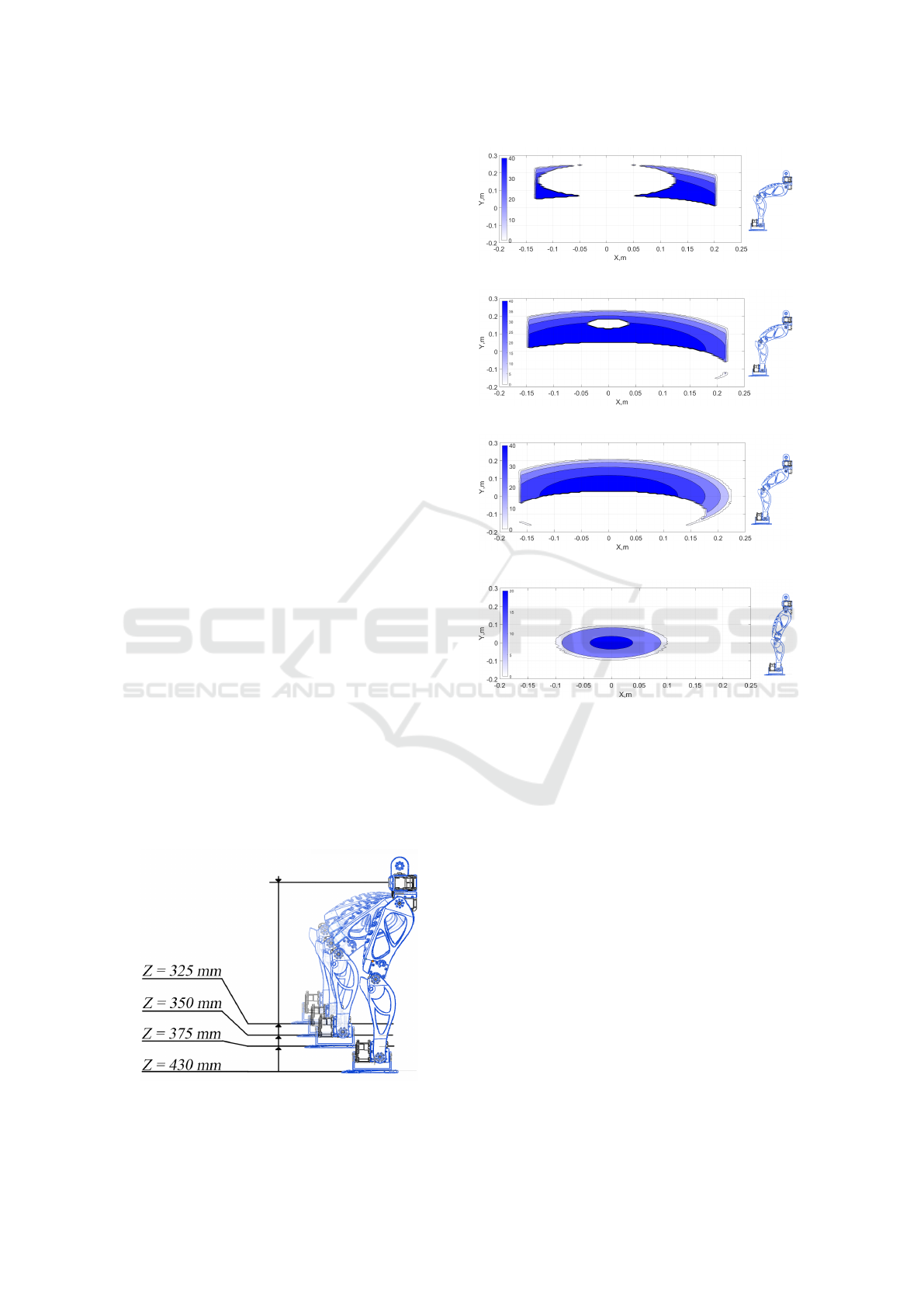
to 0 deg. in roll, pitch and yaw. The workspace

was calculated for different left foot positions rela-

tive to the torso coordinate Z: 0.325, 0.35, 0.375, and

0.43 meters (Figure 3). As a performance index for

workspace Jacobean condition number was chosen.

Condition number shows general accuracy, dexterity

of the robot, closeness to singularity.

Since the robot conﬁguration is a 6R serial chain

for one leg, workspace is limited by serial singular-

ity and mechanical joint limits. Serial singularity

can be identiﬁed by low condition number near it.

The mechanical joints limit appears as an unreach-

able area near the Y axis zero position (Hip joint lim-

its) see Figure 4a, 4b, 4c and as an ellipse inside the

workspace at small torso height (Knee joint limit) see

Figure 4a, 4b.

Figure 3: Foot positions relative to the torso coordinate Z.

(a) Distance between foot and the torso Z=325 mm.

(b) Distance between foot and the torso Z=350 mm.

(d) Distance between foot and the torso Z=430 mm.

Figure 4: Achievable foot location and condition number

with example conﬁguration.

4 STIFFNESS ANALYSIS

In real life robot mechanical components (both joints

and links) are not perfectly rigid, so the foot and

torso position can differ from the expected one un-

der the load induced my robot link weights. So if we

need an accurate robot location and stable locomo-

tion, we need to calculate these deﬂections and pos-

sibly to compensate them. This can be done by de-

veloping and analyzing robot stiffness model. This

stiffness model can be obtained using Virtual Joint

Method (VJM) (Pashkevich et al., 2011). According

to this method non-rigid manipulator links can be rep-

resented as pair of rigid link and 6 DoF virtual spring

and non-rigid actuators as perfect actuator and 1 DoF

virtual spring describing its elasticity.

In practice, the end-effector position (foot or/and

torso position) can be found from the extended geo-

ICINCO 2017 - 14th International Conference on Informatics in Control, Automation and Robotics

metric model as

t = g(q,θ) (12)

where q is the vector of actuator coordinates q =

,...,q

)

and θ the vector of virtual joint co-

ordinates θ = (θ

,θ

,...,θ

)

. Since the link weights

are the main source of deﬂections in anthropomorphic

robots, it should be also considered in the model. Ex-

ternal load caused by weight of the links can be repre-

sented as forces acting in the node-points correspond-

ing to virtual spring locations. In the simpliﬁed model

used in this paper these virtual springs take into ac-

count both link and actuator compliances. By apply-

ing principle of virtual work, the static equilibrium of

corresponding static system can be founded as (Klim-

chik et al., 2014)

(G)T

· G + J

(F)T

· F = K

· θ (13)

where the matrix J

(G)

(1)T

,..,J

(n)T

aggregates

partial Jacobians from the robot base to correspond-

ing node point with gravity load, J

(F)

is the Jaco-

bian from base of the robot to end-effector with ex-

ternal load, the vector G aggregates forces applied

in the internal nodes (caused by gravity), F is vec-

tor of external load applied to the end-effector and

= diag(K

θ1

,...,K

θn

) diagonal matrix with stiff-

ness of all virtual springs. Desired static equilibrium

conﬁguration can be found using iterative algorithm

(Klimchik et al., 2014) .

i+1

= (J

(F)

· K

−1

· J

(F)T

)

−1

· (t

i+1

− g(q,θ

(F)

· θ

− J

(F)

· K

−1

· J

(G)T

· G

)

i+1

= K

−1

(G)T

· G

+ J

(F)T

· F

i+1

)

(14)

and the Cartesian stiffness matrix K

can be computed

as follows



∗

∗ ∗





· K

−1

· J



−1

(15)

this allows us to obtain force-deﬂection relation

∆t = K

−1

· F (16)

where ∆t end-effector deﬂections, and estimate com-

pliance errors caused by gravity forces.

For the considered humanoid robot the main

source of elasticity is related to the motor and gear-

box ﬂexibility. So, for simplicity, all links are consid-

ered to be rigid while actuated joints are considered to

be deformable. Friction forces are not taken into ac-

count. According to the VJM notation 1 DoF virtual

springs will be added after each actuator.

(a) Left leg model. (b) Right leg model.

Figure 5: Robot VJM model.

For stiffness analysis of humanoid (similarly to

kinematic and dynamic analyses) two walking phases

should be addressed: single support phase (SSP) and

dual support phase (DSP). In dual support stage both

legs are on the ground. Assuming that there is no slip

between surface and robot feet, it can be represented

as parallel manipulator with two 6R serial chains. De-

ﬂections from external forces will only affect position

of robot trunk and, assuming that deﬂections too small

to move robot center of mass (CoM) out of support

polygon, do not contribute to robot stability.

Most critical stage for bipedal robot where deﬂec-

tions can have a strong effect on stability is single sup-

port stage. In this stage one of the robot legs is swing

and deﬂections caused by gravity force or/and exter-

nal load can displace swaying leg closer to the ground

or collide them. This undesired contact may lead the

robot to fall. Robot VJM model in that stage can be

introduced as two serial chains (Figure 5a and 5b).

the ﬁrst chain (Figure 5b) consist of 6 active joints

and 6 virtual joints, base ﬁxed to the surface. In addi-

tion to gravity forces G

, there are external loadings

caused by weight of upper body and swing leg. Sec-

ond chain (Figure 5a) consists of 6 active joints and

6 virtual joints, base position can be found as end-

effector position of ﬁrst chain plus deﬂections in the

end-effector of ﬁrst chain. Second chain affected only

by gravity forces G

Total deﬂection can be calculated in 3 steps:

1. Calculate deﬂection for standing leg pelvis chain

with gravity load and external load in end-effector

that correspond to pelvis (upper body) mass +

swing leg mass.

2. Calculate deﬂections for pelvis swing leg chain

with swing leg gravity load.

3. Combine deﬂections from 2 chains.

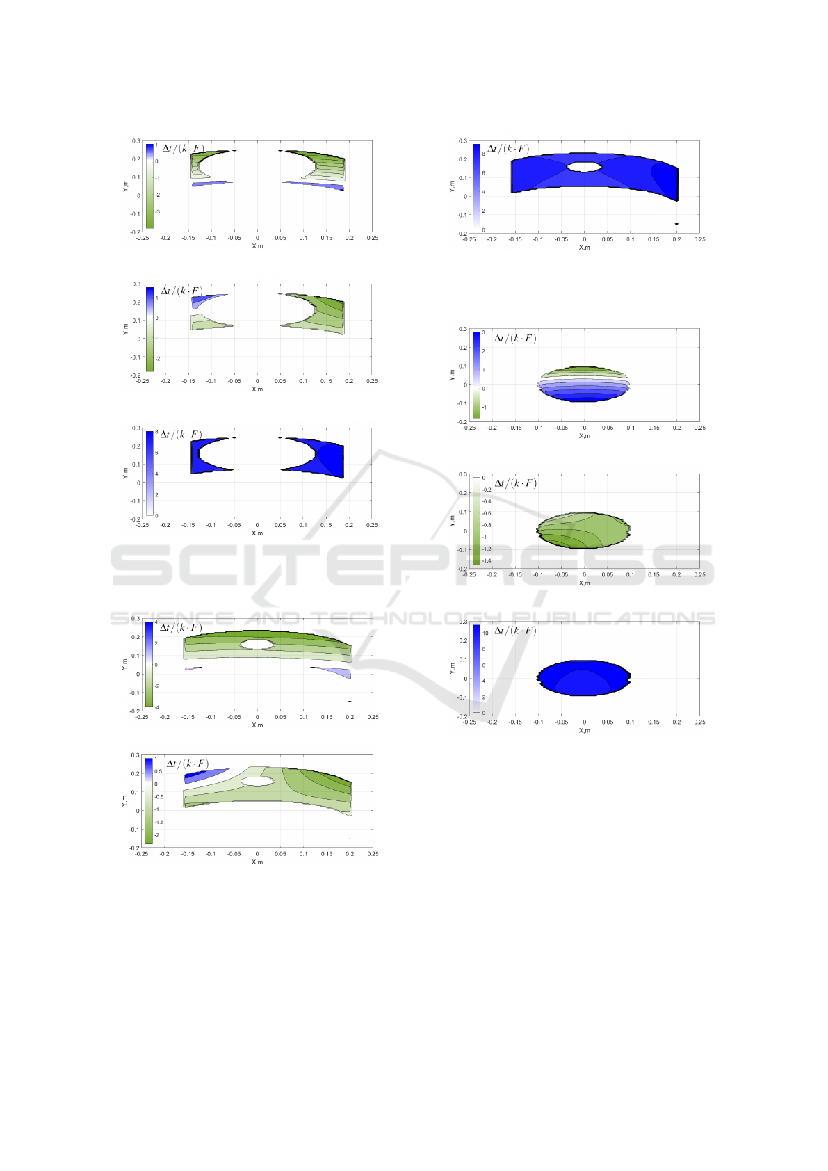
Deﬂection magnitudes for different swing leg

heights (presented in Figure 3) within the reachable

workspace shown in Figure 6a, 6b, 6c, 6d. Right

leg conﬁguration (ﬁxed on the ﬂoor) used for these

Design and Stiffness Analysis of 12 DoF Poppy-inspired Humanoid

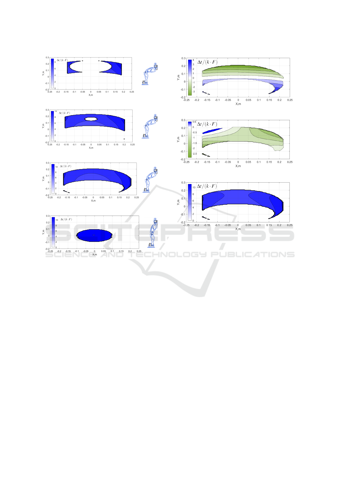
(a) Distance between foot and the torso Z=325 mm.

(b) Distance between foot and the torso Z=350 mm.

(d) Distance between foot and the torso Z=430 mm.

Figure 6: Deﬂections magnitude of the left foot for different

swing leg hight.

ﬁgures is static and all joint coordinates are equal to

zero. It is shown that deﬂections are increasing near

the border of the workspace. The minimal deﬂections

can be achieved close to (0;0) point, but this conﬁgu-

ration is not reachable by the swing leg for the heights

less than 375 mm.

Deﬂection vector components for the swing leg

high 375mm are shown in Figure 7a, 7b, 7c. Ad-

ditional ﬁgures for other leg highs are presented in

Appendix (Figures 13-16). Deﬂections in X and Y di-

rections can be positive or negative, depending on the

leg conﬁguration. This behavior is explained by shift-

ing robot center of mass. Deﬂections in Z direction

have maximum magnitude and are the most critical

ones, since they shift robot foot closer to the ground.

(a) Deﬂections in X directions.

(b) Deﬂections in Y directions.

Figure 7: Deﬂection vector components for distance be-

tween foot and the torso Z=375 mm.

5 TRAJECTORY PLANNING

The biped walking pattern was obtained using Zero

Moment Point (ZMP) preview control, proposed by

(Kajita et al., 2003). ZMP preview control allows to

obtain CoM trajectory based on ZMP-reference tra-

jectory as it is shown in Figure 8a, 8b. With CoM

trajectory and robot leg’s end-effector trajectories it

is possible to ﬁnd joint angles with inverse kinemat-

ics described previously. Trajectory generated with

this method assumes that robot links and joints are

perfectly stiff. In order to include information about

possible deﬂections to trajectory generation, external

compensation technique is required.

The following algorithm for simple off-line com-

pensation for SSP is used:

1. Generate trajectory for CoM using ZMP preview

control.

2. Calculate deﬂections in each SSP for both legs for

all points on trajectory.

3. Find new legs end effector coordinates as p

new

ICINCO 2017 - 14th International Conference on Informatics in Control, Automation and Robotics

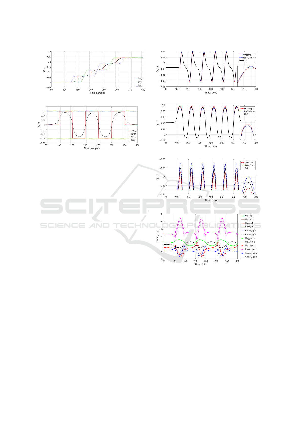
(a) Robot motion in sagittal plane.

(b) Robot motion in lateral plane.

Figure 8: Walking pattern generated by preview control.

p − ∆t.

4. Recalculate inverse kinematics for new trajecto-

ries.

For simulation following walking pattern genera-

tion parameters were used:

• Step size - 6 cm

• CoM height - 43 cm

• Number of step phases = 15 (for demonstration)

• Control frequency - 50 Hz

• Leg lift - 5 cm

• Dual support phase - 20%.

Ankle trajectories in X, Y, Z plane are shown in

Figure 9a, 9b, 9c respectively. Deﬂections in X and

Y planes are small compared to Z. Table 6 shows nor-

malized position error value with and without com-

pensation. High improvement factor can be explained

by the linearity of the model. Joint trajectories with

and without compensation are presented in Figure 9d.

Knee, hip and ankle joints rotating around Y axis have

the most essential changes due to compensation, since

they correspond to movements of end-effector in Z di-

rection, where deﬂections have maximal magnitude.

Difference between reference and compensated con-

trol signal for left leg ankle shown in Figure 10. Since

only the SSP is considered for compensation, error for

intervals where the left leg placed on the ground are

equal to zero. Lower amplitude of error in the ﬁrst

step can be explained by the fact that ﬁrst step is ac-

tually a half-step.

(a) Ankle position X.

(b) Ankle position Y.

(d) Joint angles.

Figure 9: reference and non-compensated spatio-temporal

joint trajectories for robot gait.

Total stability improvement for the biped robot

can be observed by looking at ZMP position and

its position error compared to reference ZMP trajec-

tory. Trajectories obtained from preview control (Fig-

ure 8a, 8b) were examined with the robot model in

V-REP, after that ZMP trajectory were obtained from

virtual sensors. Figure 11a, 11b present ZMP po-

sition in Y and X plane over time. ZMP position

without compensation has a noticeable peak at the

point where foot of the robot contacted with ground

surface and because of deﬂections it’s happen before

DSP deﬁned by the algorithm. This cause robot to

stumble and move its ZMP closer to the edges of sup-

Design and Stiffness Analysis of 12 DoF Poppy-inspired Humanoid

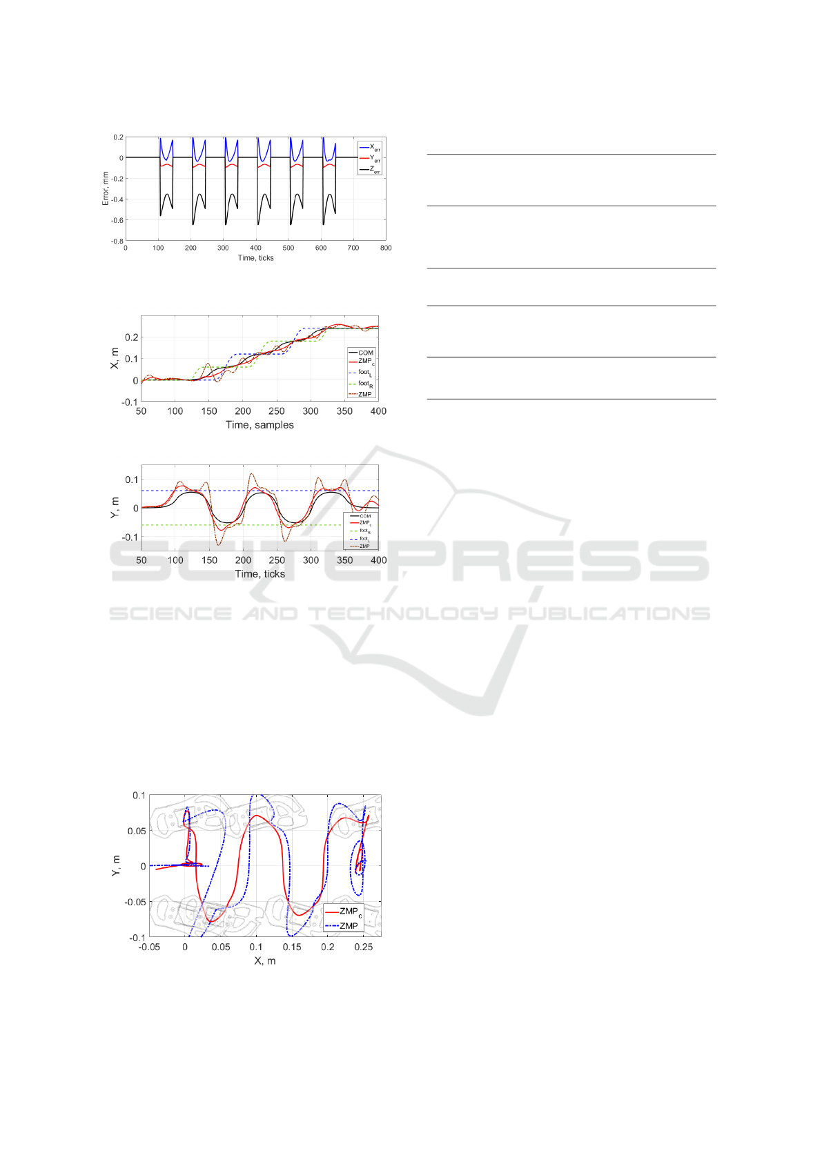
Figure 10: Error between reference and compensated tra-

jectory for ankle position.

(a) Robot motion in sagittal plane.

(b) Robot motion in lateral plane.

Figure 11: Simulated robot walking trajectories with and

without compensation in V-REP.

port polygon. Maximum amplitude of difference be-

tween compensated/non-compensated and reference

ZMP position presented in Table 7. Figure 12 intro-

duce ZMP position with and without compensation

in XY plane (top view). Using compensation of de-

ﬂections allowed to reduce error by 61% in X plane

(forward movements) and by 73% in Y plane (side

movements).

Figure 12: Simulated biped robot ZMP with and without

compensation in XY plane.

Table 6: Maximum end-effector position errors.

Error before

compensation

(∆t/(k · F))

Error after

compensation

(∆t/(k · F))

X 3.06 0.19 93.8

Y 2.22 0.09 95.9

Z 10.41 0.65 93.7

Table 7: Maximum ZMP errors compared to reference.

Error before

compensation

(mm)

Error after

compensation

(mm)

X 51.62 20.04 61.2

Y 68.41 18.27 73.3

The simulated ZMP trajectory was also validated

on the real 3D-printed robot prototype. During tests

robot demonstrated stable walking capability with

off-line generated joint trajectories.

6 DISCUSSION

Stiffness modeling for bipedal robots allow to reduce

position error for the robot legs, especially in Z di-

rection, that is critical for stable walking ability. In

this work only the joint compliance was used, but

it’s possible to further improve stiffness model by

implementing a link stiffness model in addition to

joint model. This improved model will allow to in-

crease error reduction depending on the robot struc-

ture (Klimchik et al., 2015). Link compliance is more

valuable for full-size humanoid robots, where mass

of the robot parts is relativity high. The robot used in

this work has small size and low mass and link com-

pliance could be ignored. But in the same time ma-

terial (ABS - plastic) has quite low Young’s modulus

value and process (Fused deposition modeling) used

for robot link creation will reduce total stiffness of the

robot links. Further experiments required in order to

understated how implementing of more complicated

model will increase performance of walking motion.

Another way of increasing error reduction is imple-

mentation of non-linear model that could further de-

crease error.

The current algorithm calculates deﬂection off-

line. For humanoid robot that could constantly re-

calculates moving trajectory based on its environment

on-line method should be implemented by computing

possible deﬂection each control cycle or by using pre-

viosly calculated patterns.

ICINCO 2017 - 14th International Conference on Informatics in Control, Automation and Robotics

7 CONCLUSIONS

The main goal of this work was to design low-

cost bipedal anthropomorphic robot, provide stiff-

ness analysis and implement error compensation tech-

nique. The biped robot was designed based on open

source Poppy Humanoid project with 10 DoF lower

limbs, but with enhancing their mechanical structure

and functionality with additional DoF at the ankle.

The robot’s lower body was modeled in V-REP sim-

ulator and prototyped using 3D printing technology.

Despite increasing DoF relative to Poppy humanoid,

we succeeded to reduce overall cost using hobby ser-

vomotors, inexpensive fabrication methods and cost-

efﬁcient electronics components. As far as the cur-

rent robot design has a non-spherical hip joint, which

does not allow to use an analytical solution for the

inverse kinematics, we computed inverse kinematics

using hybrid and numerical methods. Stiffness model

of the robot was obtained using VJM for single sup-

port phase and main source of compliance in the robot

joints. Integration of stiffness model into gait pattern

generation algorithm allowed us to compensate de-

ﬂections caused by link weights. These trajectories

were examined both with the robot model in V-REP

simulator and on the real 3D-printed lower body pro-

totype. The results of experiments demonstrated sta-

ble walking capability of the designed Poppy-inspired

humanoid with 12 DoF lower limbs.

Future work includes deep consideration of mo-

tion processes, creation and implementation of on-

line trajectory generation and compensation, using

stiffness model along with the variable stiffness ac-

tuators. For hardware part the main future tasks are

to enhance and to produce lower limbs with a higher

motion range, passive/active joints with spring sup-

port, and to design robots upper body.

ACKNOWLEDGEMENTS

This research has been suppotred by the grant of Rus-

sian Ministry of Education and Science 2017-14-576-

0053-7882 and Innopolis University

REFERENCES

Buss, S. R. (2004). Introduction to inverse kinematics with

jacobian transpose, pseudoinverse and damped least

squares methods. IEEE Journal of Robotics and Au-

tomation, 17(1-19):16.

Cisneros Lim

on, R., Ibarra Zannatha, J. M., and Ar-

mada Rodriguez, M. A. (2013). Inverse kinematics of

a humanoid robot with non-spherical hip: a hybrid al-

gorithm approach. International Journal of Advanced

Robotic Systems, 10:1–13.

Craig, J. J. (2005). Introduction to robotics: mechanics and

control, volume 3. Pearson Prentice Hall Upper Sad-

dle River.

Ferro, F. and Marchionni, L. (2014). Reem: A humanoid

service robot. In ROBOT2013: First Iberian Robotics

Conference, pages 521–525. Springer.

Gouaillier, D., Hugel, V., Blazevic, P., Kilner, C., Mon-

ceaux, J., Lafourcade, P., Marnier, B., Serre, J., and

Maisonnier, B. (2009). Mechatronic design of nao hu-

manoid. In Robotics and Automation, 2009. ICRA’09.

IEEE International Conference on, pages 769–774.

IEEE.

Ha, I., Tamura, Y., Asama, H., Han, J., and Hong, D. W.

(2011). Development of open humanoid platform

darwin-op. In SICE Annual Conference (SICE), 2011

Proceedings of, pages 2178–2181. IEEE.

Jazar, R. N. (2010). Theory of applied robotics: kinematics,

dynamics, and control. Springer Science & Business

Media.

Kajita, S., Kanehiro, F., Kaneko, K., Fujiwara, K., Harada,

K., Yokoi, K., and Hirukawa, H. (2003). Biped

walking pattern generation by using preview control

of zero-moment point. In Robotics and Automa-

tion, 2003. Proceedings. ICRA’03. IEEE International

Conference on, volume 2, pages 1620–1626. IEEE.

Khusainov, R., Shimchik, I., Afanasyev, I., and Magid, E.

(2015). Toward a human-like locomotion: Modelling

dynamically stable locomotion of an anthropomorphic

robot in simulink environment. In Informatics in Con-

trol, Automation and Robotics (ICINCO), 2015 12th

International Conference on, volume 02, pages 141–

148.

Klimchik, A., Chablat, D., and Pashkevich, A. (2014). Stiff-

ness modeling for perfect and non-perfect parallel ma-

nipulators under internal and external loadings. Mech-

anism and Machine Theory, 79:1–28.

Klimchik, A., Furet, B., Caro, S., and Pashkevich, A.

(2015). Identiﬁcation of the manipulator stiffness

model parameters in industrial environment. Mech-

anism and Machine Theory, 90:1–22.

Lapeyre, M., N’Guyen, S., Le Falher, A., and Oudeyer,

P.-Y. (2014). Rapid morphological exploration with

the poppy humanoid platform. In 2014 IEEE-RAS In-

ternational Conference on Humanoid Robots, pages

959–966. IEEE.

Lapeyre, M., Rouanet, P., and Oudeyer, P.-Y. (2013a).

Poppy humanoid platform: Experimental evaluation

of the role of a bio-inspired thigh shape. In 2013 13th

IEEE-RAS International Conference on Humanoid

Robots (Humanoids), pages 376–383. IEEE.

Lapeyre, M., Rouanet, P., and Oudeyer, P.-Y. (2013b). The

poppy humanoid robot: Leg design for biped locomo-

tion. In 2013 IEEE/RSJ International Conference on

Intelligent Robots and Systems, pages 349–356. IEEE.

Pashkevich, A., Klimchik, A., and Chablat, D. (2011).

Enhanced stiffness modeling of manipulators with

Design and Stiffness Analysis of 12 DoF Poppy-inspired Humanoid

passive joints. Mechanism and machine theory,

46(5):662–679.

Peiper, D. L. (1968). The kinematics of manipulators under

computer control. Technical report, DTIC Document.

Rohmer, E., Singh, S. P., and Freese, M. (2013). V-rep:

A versatile and scalable robot simulation framework.

In 2013 IEEE/RSJ International Conference on Intel-

ligent Robots and Systems, pages 1321–1326. IEEE.

Sakagami, Y., Watanabe, R., Aoyama, C., Matsunaga, S.,

Higaki, N., and Fujimura, K. (2002). The intelligent

asimo: System overview and integration. In Intelli-

gent Robots and Systems, 2002. IEEE/RSJ Interna-

tional Conference on, volume 3, pages 2478–2483.

IEEE.

Siciliano, B. and Khatib, O. (2008). Springer handbook of

robotics. Springer Science & Business Media.

Yamaguchi, J., Soga, E., Inoue, S., and Takanishi, A.

(1999). Development of a bipedal humanoid robot-

control method of whole body cooperative dynamic

biped walking. In Robotics and Automation, 1999.

Proceedings. 1999 IEEE International Conference on,

volume 1, pages 368–374. IEEE.

APPENDIX

Analytical Solution for Inverse Kinematic

In the sagittal plane (Figure 2b) we consider lengths

, Z

and l

The position of the ankle T

, T

can be obtained

from the inverse matrix of T 6 ∗ T 7 (1).

T 1 ∗ T 2 ∗ T 3 ∗ T 4 ∗ T 5 = T F ∗ (T 6 ∗ T 7)

−1







∗ ∗ ∗ T x + z6 · r13

∗ ∗ ∗ Ty + z6 · r23

∗ ∗ ∗ T z + z6 · r33

0 0 0 1







(17)

Then ﬁnd distance l

)

= (T

+ z

· r

)

+ (T

+ z

· r

)

+ z

· r

)

(18)

The knee angle q4 can be calculated from the law

of cosines

q4 = cos

−1



− z3

− z4

2 · z3 · z4



(19)

Lengths l

06yz

and l

05yz

can be found in the frontal

plane (Figure 2a).

06yz

(T F

−1

(2,4))

+ (T F

−1

(3,4))

(20)

05yz

(T F

−1

(2,4))

+ (T F

−1

(3,4) − z6)

(21)

The ankle roll angle can be calculated by the law

of cosine

q6 = cos

−1

06yz

− l

05yz

− z6

2·l

05yz

· z6

(22)

T 1 ∗ T 2 ∗ T 3 ∗ T 4 = T F ∗ (T 5 ∗ T 6 ∗ T 7)

−1

(23)

Find q1 and q2 from (23), by comparing right

hand side (RHS) and left hand side (LHS) equations.

If we inverse T 1 ∗ T 2, T 6 ∗ T 7 and multiply them

with TF

T 3 ∗T 4∗T 5 = (T 1 ∗ T 2)

−1

∗T F ∗(T 6 ∗ T 7)

−1

(24)

Then RHS and LHS equations will be:

RHS =







∗ ∗ ∗ A

∗ ∗ ∗ B

∗ ∗ ∗ ∗

0 0 0 1







(25)

where

A = −T x · sin (q2)sin (q1)+

Ty · cos (q2) sin(q1) − T z · cos(q1)−

z6(r13 · sin(q1)sin (q2)−

r23 · cos(q2)sin (q1) +r33 · cos (q1))

(26)

B = −T x · cos (q2) − Ty · sin (q2)−

z6(r13 · cos(q2) + r23 · sin (q2))

(27)

LHS =







∗ ∗ ∗ C

∗ ∗ ∗ D

∗ ∗ ∗ ∗

0 0 0 1







(28)

where

C = (z3 + z4 · cos(q4))cos (q3)−

z4 · sin(q4)sin(q3)

(29)

D = z4 · sin(q4) cos (q3)+

(z3 + z4 · cos(q4)) sin(q3)

(30)

Solve it for q3 and then ﬁnd q5 from known q3

and q4. Final equations for 6 DoF leg presented in

section 3.2.1

Deﬂections Maps for Biped Robot

Figures 13-16 shows X, Y, Z deﬂection vector com-

ponents for the left leg hight is presented in Figure 3.

ICINCO 2017 - 14th International Conference on Informatics in Control, Automation and Robotics

(a) Deﬂections in X directions.

(b) Deﬂections in Y directions.

Figure 13: Deﬂection vector components for distance be-

tween foot and the torso Z=325 mm.

(a) Deﬂections in X directions.

(b) Deﬂections in Y directions.

Figure 14: Deﬂection vector components for distance be-

tween foot and the torso Z=350 mm.

(a) Deﬂections in X directions.

(b) Deﬂections in Y directions.

Figure 15: Deﬂection vector components for distance be-

tween foot and the torso Z=430 mm.

Design and Stiffness Analysis of 12 DoF Poppy-inspired Humanoid

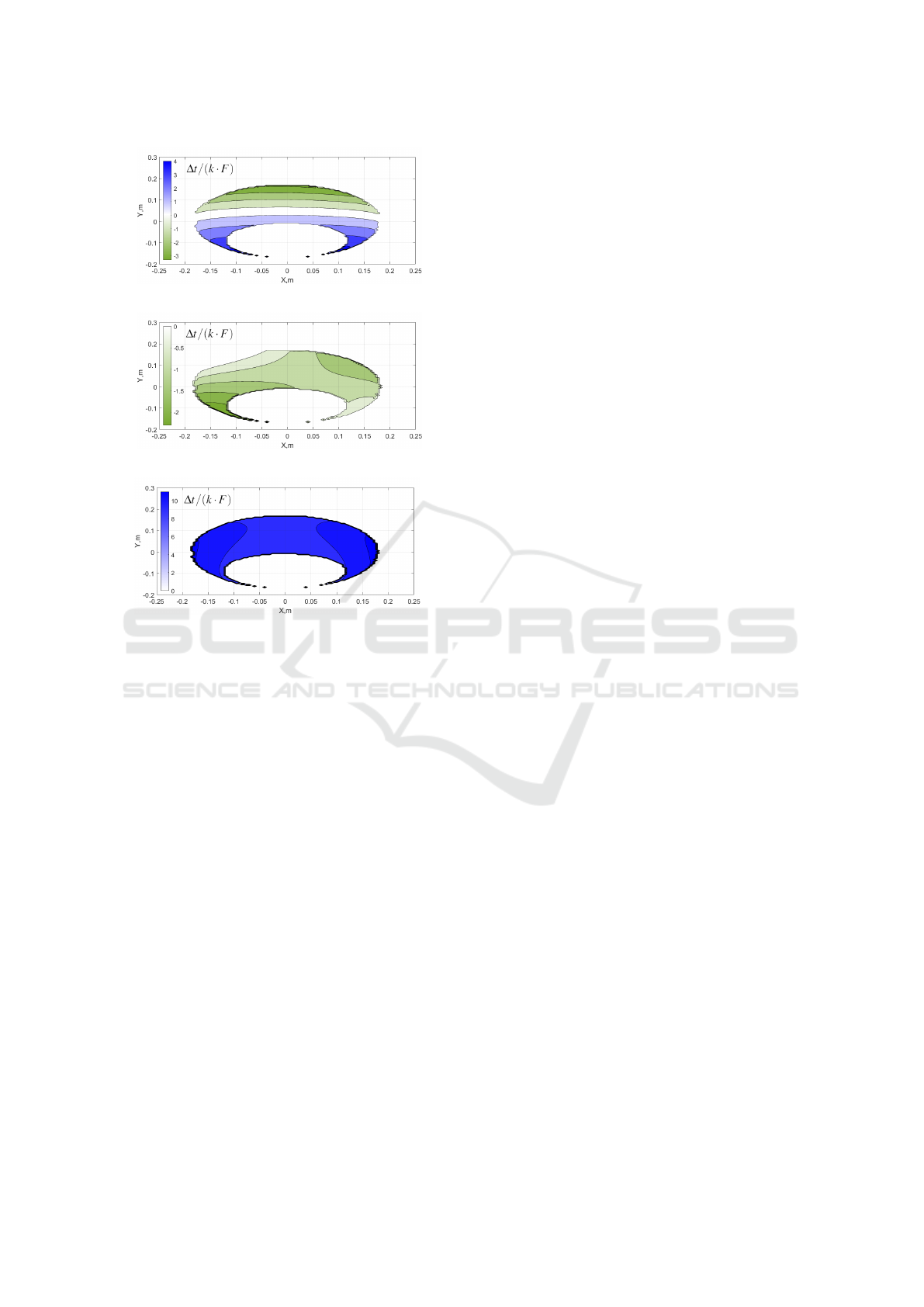
(a) Deﬂections in X directions.

(b) Deﬂections in Y directions.

Figure 16: Deﬂection vector components for distance be-

tween foot and the torso Z=400 mm.

ICINCO 2017 - 14th International Conference on Informatics in Control, Automation and Robotics