
C2-continuous Path Planning by Combining Bernstein-B
´
ezier Curves
Gregor Klanˇcar, Saˇso Blaˇziˇc and Andrej Zdeˇsar
Faculty of Electrical Engineering, University of Ljubljana, Trˇzaˇska 25, SI-1000, Ljubljana, Slovenia
Keywords:
Path Planing, Bernstein-B´ezier (BB) Curve, Splines, Optimal Velocity Profile, Wheeled Mobile Robot.
Abstract:
This work proposes fifth order Bernstein-B´ezier (BB) curve segments to be used in path planning approaches.
The combined path consists of BB spline sections with continuous second derivative in connections which
means that the path curvature is continuous and feasible for wheeled robot to drive on. To further minimize the
travelling time on this path a velocity profile is optimized by considering acceleration and velocity constraints.
1 INTRODUCTION
Path planning in a known environment with obsta-
cles presented by its map is very common task in
mobile robot applications and has been widely stud-
ied in (Schwartz and Sharir, 1990), (Latombe, 1991),
(LaValle, 2006). Environment usually is decomposed
to cells by some algorithm like regular rectangular
grid, quad trees, random sampling-based methods
and the like (LaValle, 2006), (Choset et al., 2005),
(Klanˇcar et al., 2017). Among those cells an optimal
collision-free path need to be find connecting current
robot position and the goal location. The most com-
monly used is A star algorithm which returns opti-
mal sequence of connected straight lines through the
cells centers towards the goal location. Such com-
bined path does not have continuous first and second
derivative (is not C1 and C2 continuous). C1 not con-
tinuous path means that the robot following this path
would have step changes of orientation while C2 dis-
continuous means that the robot angular velocity or
also path curvature κ has step changes. Therefore the
calculated path need to be smoothed to become feasi-
ble for the robot to follow it. The first studies to obtain
the shortest smooth paths consisting of straight lines
and circular arc was performed by (Dubins, 1957).
His paths are only C1 continuous as they have dis-
continuous curvature.
Some possible smoothing approaches are as fol-
lows. A funnel algorithm is proposed in (Kallmann,
2005) to further optimize the path inside the corri-
dor defined by the cells contained on the optimal
path. For path optimization and smoothing inside
the corridor a Fast marching method (Sethian, 1999)
can be applied or smooth path generation using B-
splines as in (Berglund et al., 2011). Several path
smoothing ideas using local nonlinear optimization
and non-parametric optimization using conjugated-
gradient solution are described in (Dolgov et al.,
2008). Often sharp transitions on the path e.g.
corners are smoothed by inserting smooth paramet-
ric curves such as circular arcs (Yang and Wushan,
2015), Bezier curves (Choi et al., 2010), clothoids
or higher order polynomials (Brezak and Petrovi´c,
2014), (Sencer et al., 2015) enabling C2 continuous
transitions.
Path smoothing is often not integrated in path
planning but is usually done after the optimal path
is found. This however requires additional collision
checks and can influence path optimality. Several lo-
cal path planners ware proposed to find smooth path
sections between initial and target pose in obstacles
free space as in (Chen et al., 2014) where four order
B´ezier curves are applied to obtain continuous and
bounded curvature path. However finding collision
safe, smooth and optimal path in complex environ-
ments with obstacles remains a challenging task. To
cope with it a hybrid A star algorithm (Dolgov et al.,
2008) was proposed which can find drivable reference
path for wheeled robots. The path usually consists of
curves obtained by setting constant robot commands.
This work addresses continuous path planing
problem where we suggest the path to be composed of
Bernstein-B´ezier curves with continuous velocity and
curvature transitions. The obtained path can there-
fore be directly driven by wheeled mobile robots. To
achieve the shortest travelling time a driving veloc-
ity optimization approach is performed by consider-
ing robot capabilities. The main idea is to drive with
maximal allowed accelerations and velocity to avoid
254
Klan
ˇ
car, G., Blaži
ˇ
c, S. and Zdešar, A.
C2-continuous Path Planning by Combining Bernstein-Bézier Curves.
DOI: 10.5220/0006406602540261
In Proceedings of the 14th International Conference on Informatics in Control, Automation and Robotics (ICINCO 2017) - Volume 2, pages 254-261
ISBN: Not Available
Copyright © 2017 by SCITEPRESS – Science and Technology Publications, Lda. All rights reserved
wheel slipping. Several path and velocity planing ex-
amples are illustrated.
Main paper contributions are two. The first is the
definition of fifth order B´ezier curve sections which
can easily be applied to compose a C2 continuous
path in some path planning applications. The second
contribution is optimal velocity profile calculation ap-
proach for a spline path consisting of more B´ezier
curves.
2 PATH COMPOSITION IN
CONTINUOUS PATH PLANING
Resulting path in most path planing approaches is
composed of path sections which are continuously
joined. Usually the search is done in discrete space
by discretization of all possible robot poses (e.g. grid-
based presentation of environment) to a finite set.
Other very often used approach is to discretize input
commands while the pose remains continuously de-
fined as it is usually done in continuous path planing
approaches (e.g. hybrid A star). The former can be
applied to differential drive robot which commands
are linear velocity v(t) and angular velocity ω(t). In
each node (robot pose) the path planing algorithm ex-
pands the search in a predefined number of travel-
ling curves obtained by setting some constant trans-
lational velocity v(t) = v
CONST
and angular velocity
ω(t) ∈ [ω
MIN
,··· ,0,··· , ω
MAX
]. The path sections
therefore have circular shape and the final robot pose
(x(t
F
), y(t
F
), ϕ(t
F
)) at time t
F
= t
S
+ ∆t is obtained
by integration
x(t
F
) =
R
t
F
t
S
v(t)cos(ϕ(t))dt + x(t
S
)
y(t
F
) =
R
t
F
t
S
v(t)sin(ϕ(t))dt + y(t
S
)
ϕ(t
F
) =
R
t
F
t
S
ω(t)dt + ϕ(t
S
)
(1)
which exact solution is
x(t
F
) = x(t
S
) +
∆s
∆ϕ
(sin(ϕ(t
S
) + ∆ϕ)− sin(ϕ(t
S
))
y(t
F
) = y(t
S
) −
∆s
∆ϕ
(cos(ϕ(t
S
) + ∆ϕ)− cos(ϕ(t
S
))
ϕ(t
F
) = ϕ(t
S
) + ∆ϕ
(2)
where t
S
is starting time, t
F
is final time, ∆t time
increment for the path section, ∆s = v∆t is travelled
distance and ∆ϕ = ω∆t change of robot orientation.
An example of search expansion using circular
paths (e.g. as in hybrid A star) expansion tree
(where x(0) = y(0) = 0, ϕ(0) = π/4, v = 0.5, ω ∈
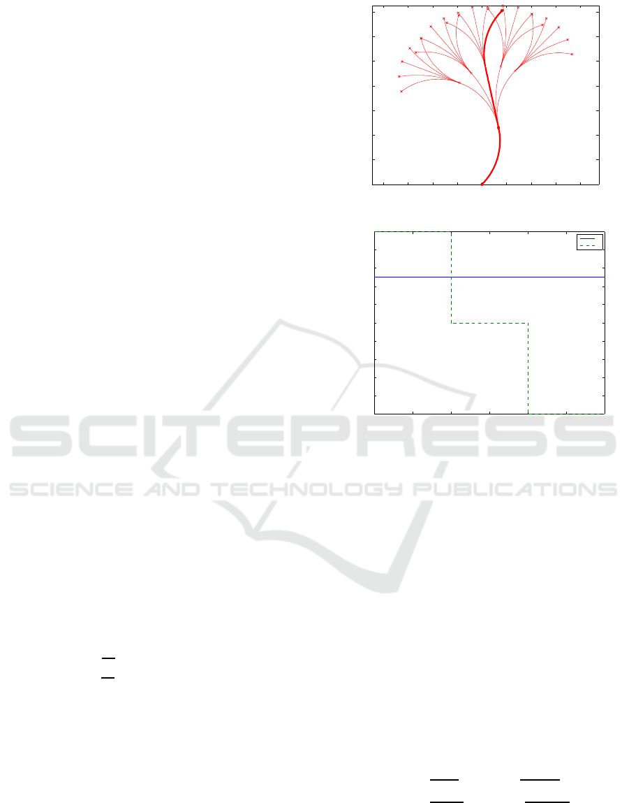
[−1,−0.5,0, 0.5,1] and ∆t = 1, ) is given in Fig. 1.
To follow the thick path in Fig. 1 robot controls
need to be as shown in Fig. 2 which obviously is not
C2 continuous because ω(t) is discontinuous.
−0.8 −0.6 −0.4 −0.2 0 0.2 0.4 0.6 0.8
0
0.2
0.4
0.6
0.8
1
1.2
1.4
x[m]
y[m]
Figure 1: Search expansion using circular paths.
0 0.5 1 1.5 2 2.5 3
−1
−0.8
−0.6
−0.4
−0.2
0
0.2
0.4
0.6
0.8
1
t[s]
v[m/s], ω [1/s]
v
ω
Figure 2: Differential drive robot control signal to follow
thick path in Fig. 1.
To have feasible planed path for the robot a C2
continuous Bernstein-B´ezier (BB) curves are pro-
posed as follows. To achieve C2 continuous path a
proper spline of two connecting BB curves need to be
achieved.
To achieve this at least forth order BB curve r(λ)
need to be selected. It is defined by five control points
P
i
= [x
i
,y
i
]
T
, i ∈= 0,1,··· ,4 as follows
r(λ) = (1− λ)
4
P
0
+ 4λ(1− λ)
3
P
1
+6λ
2
(1− λ)
2
P
2
+ 4λ
3
(1− λ)P
3
+ λ
4
P
4
(3)
where λ is a normalized time (0 ≤ λ ≤ 1). In this
section without loss of generality assume λ = t. A C2
spline of two BB curves r
j
and r
j+1
is obtained by
setting the following conditions
lim
λ→1
r
j
(λ) = lim
λ→0
r
j+1
(λ)
lim
λ→1
dr
j
(λ)
dλ
= lim
λ→0
dr
j+1
(λ)
dλ
lim
λ→1
d
2
r
j
(λ)
d
2
λ
= lim
λ→0
d
2
r
j+1
(λ)
d
2
λ
(4)
saying that the end of the curve j and the start of
the curve j+1 as well as their first and second deriva-
tive need to coincide. From (4) the conditions for se-
lection of the j + 1 BB curve control points P
i, j+ 1
re-
C2-continuous Path Planning by Combining Bernstein-Bézier Curves
255
lated to control points of j-th curve (P
i, j
) selection
reads
P
0, j+1
= P
4, j
P
1, j+1
= 2P
4, j
− P
3, j
P
2, j+1
= 4P
4, j
− 4P
3, j
+ P
2, j
(5)
To have similar spread of paths sections as in Fig.
1 the last control point P
4, j+1
of BB curves is cal-
culated using final position x(t
F
), y(t
F
) calculated by
(2). While final curve orientation is achieved by set-
ting P
3, j+1
according to the final orientation ϕ(t)
P
3, j+1
= P
4, j+1
+
1
4
v
cos(ϕ(t
F
) + π)
sin(ϕ(t
F
) + π)
(6)
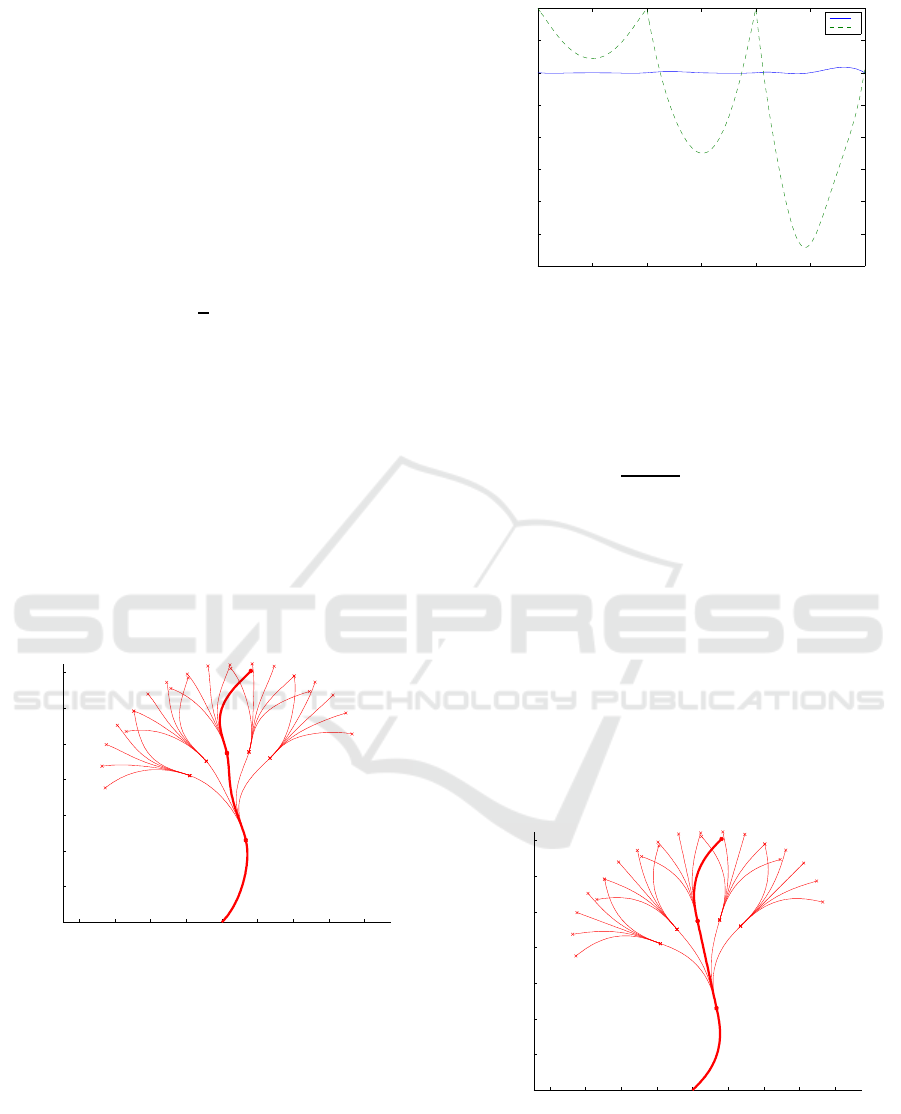
Path expansion during path-planing using BB
curves is shown in Fig. 3. Initial points of the first
BB curve are
P
0, j=1
= [x(0),y(0)]
T
P
1, j=1
= P
0, j=1
+ 0.25v[cosϕ(0),sinϕ(0)]
T
P
2, j=1
= 0.5P
1, j=1
+ 0.5P
3, j=1
while P
3, j=1
and P
4, j=1
are defined considering
next curve segments and relations (5). The obtained
graph tree of paths has the same spread as in Fig. 1
but with continuous second derivative as seen in Figs.
3 and 4.
−0.8 −0.6 −0.4 −0.2 0 0.2 0.4 0.6 0.8
0
0.2
0.4
0.6
0.8
1
1.2
1.4
x[m]
y[m]
Figure 3: Search expansion using C2 continuous BB paths.
However having a closer look of Figs. 3 and 4
one can observe some unnecessary winding of the re-
sulting paths. This is easily seen in the second path
section which start and end direction are the same but
the path between the start and end point is not straight
as it could be. To improve this behaviour BB curves
of the fifth order are used
r(λ) = (1− λ)
5
P
0
+ 5λ(1− λ)
4
P
1
+10λ
2
(1− λ)
3
P
2
+ 10λ
3
(1− λ)
2
P
3
+5λ
4
(1− λ)P
4
+ λ
5
P
5
(7)
0 0.5 1 1.5 2 2.5 3
−2.5
−2
−1.5
−1
−0.5
0
0.5
1
1.5
t[s]
v[m/s], ω[1/s]
v
ω
Figure 4: Differential drive robot control signal to follow
thick path in Fig. 3. Angular velocity is continuous while
translational velocity is similar to that in Fig. 2.
and additional conditions besides those in (4) is
defined to obtain zero angular velocity and zero tan-
gential acceleration at the curve end. This is defined
as follows lim
λ→1
dϕ
j+1
(λ)
dλ
= 0 and lim
λ→1
a
t, j+1
= 0.
The resulting control points reads
P
0, j+1
= P
5, j
P
1, j+1
= 2P
5, j
− P
4, j
P
2, j+1
= 4P
5, j
− 4P
4, j
+ P
3, j
P
3, j+1
= 2F− E
P
4, j+1
= F
P
5, j+1
= E
(8)
where E = [x(t),y(t)]
T
, F = E +
0.2v[cos(ϕ(t) + π),sin(ϕ(t) + π)]
T
and control
point P
3, j+1
satisfies the additional two conditions.
Graph tree of the obtained paths is C2 continuous and
more smooth as seen in Figs. 5 and 6.
−0.8 −0.6 −0.4 −0.2 0 0.2 0.4 0.6 0.8
0
0.2
0.4
0.6
0.8
1
1.2
1.4
x[m]
y[m]
Figure 5: Search expansion using C2 continuous BB paths
of fifth order.
The obtained combined path is therefore feasi-
ble for the robot to follow. It is smooth with con-
tinuous control velocities, continuous path curvature
ICINCO 2017 - 14th International Conference on Informatics in Control, Automation and Robotics
256
0 0.5 1 1.5 2 2.5 3
−1.5
−1
−0.5
0
0.5
1
1.5
t[s]
v[m/s], ω[1/s]
v
ω
Figure 6: Differential drive robot control signal to follow
thick path in Fig. 5.
and therefore is appropriate for optimal path-planing
methods.
3 OPTIMAL PATH AND
OPTIMAL VELOCITY
PROFILE
The problem of finding shortest time optimal path
in the environment with obstacles considering robot
capabilities and obstacles is computationally intense.
Thereforeit usually is decoupled to a problem of find-
ing a feasible collision safe path in discrete search
space (e.g. A star algorithm) and then followed by
some additional optimization.
Supposing the combined path from BB curves
given in section 2 is the output of some path find-
ing algorithm. The path is collision safe and close
to being spatially optimal (depending on path dis-
cretization, e.g. number of defined successor curve
segments). It additionally has continuous curvature
which allow optimization of its velocity profile to
achievealso shortesttravelling time. Optimal velocity
profile can be calculated as follows.
The curve is defined spatially by a schedule pa-
rameter u as x
p
(u), y
p
(u), u ∈ [0,n] where n is the
number of BB curves in the spline. The j-th curve
of the spline is defined by scheduling parameter val-
ues u ∈ ( j − 1, j] and maps to the j-th BB curve nor-
malized time λ
j
= u− j + 1 (valid if j − 1 ≤ u ≤ j).
To optimize the velocity profile of the given path one
need to consider robot capabilities such as maximum
velocity and acceleration which provide safe driving
without slip of the wheels. To obtain the trajectory
x(t), y(t) from the spatially given path one need to
define the schedule u = u(t). The curve translational
velocities v, angular velocity ω and curvature κ are
v(t) =
q
x
′
p
(u(t))
2
+ y
′
p
(u(t))
2
˙u(t) = v
p
(u) ˙u(t)
(9)
ω(t) =
x
′
p
(u(t))y
′′
p
(u(t))−y
′
p
(u(t))x
′′
p
(u(t))
x
′
p
(u(t))
2
+y
′
p
(u(t))
2
˙u(t)
= ω
p
(u) ˙u(t)
(10)
κ(t) =
x
′
p
(u(t))y
′′
p
(u(t)) − y
′
p
(u(t))x
′′
p
(u(t))
x
′
p
(u(t))
2
+ y
′
p
(u(t))
2
3/2
= κ
p
(u)
(11)
where primes stand for derivatives with respect to u,
while dots stand for derivatives with respect to t.
Main idea is to limit overall acceleration
a =
q
a
2
t
+ a
2
r
(12)
which result is robot motion without wheel slip-
ping (Lepetiˇc et al., 2003). Where translational ac-
celeration is a
t
=
dv
dt
and radial acceleration is a
r
=
vω = v
2
κ. Maximal tangential a
MAXt
and radial ac-
celeration a
MAXr
(can be different) define the overall
acceleration to be somewhere on the ellipse
a
2
t
a
2
MAXt
+
a
2
r
a
2
MAXr
= 1 (13)
for time-optimal planning.
Robot translational velocity need to be the slow-
est in the curve points u = u
TPi
(i = 1,··· ,n
TP
, n
TP
is number of TPs), called turn points (TP) where ab-
solute value of the curvature is locally maximal. For
all located TPs it holds: a
t
(u
TPi
) = 0 and a
r
u
TPi
=
a
MAXr
. Meaning that translational velocity in TP is
defined as follows
v
p
(u
TPi
) =
r
a
MAXr
|κ(u
TPi
)|
(14)
and robot therefore need to decelerated before
each TP and accelerate after each TP considering ac-
celeration constraint (13). For each TP a candidate
maximum velocity profile is computed and the final
optimal velocity profile solution is obtained by min-
imizing all TPs candidate velocity profile. Because
v(t) and v
p
(u) are proportional dependant with time
derivative of the schedule ˙u(t) one can minimize the
derivative of the schedule ˙u(t) instead which is com-
puted as follows. From acceleration constraint (13)
considering
a
r
(t) = v
2
p
(u)κ
p
(u) ˙u
2
(t) (15)
and
a
t
(t) =
dv
p
(u)
du
˙u
2
(t) + v
p
(u) ¨u(t) (16)
C2-continuous Path Planning by Combining Bernstein-Bézier Curves
257

follows the optimal schedule differential equation
¨u = ±a
MAXt
s
1
v
2
p
−
v
2
p
κ
2
p
˙u
4
a
2
MAXr
−
dv
p
du
1
v
2
p
˙u
2
(17)
which solution is found numericallyby integrating
backward and forward in time from the TPs. Minus
applies when deaccelerating (integrating backward in
time) and positive sign when accelerating (integrating
forward in time). Initial conditions u(t) and ˙u are de-
fined by known position of TPs u
TPi
and from
˙u|
TPi
=
r
a
MAXr
v
2
p
(u
TPi
)κ
p
(u
TPi
)
(18)
knowing that radial acceleration in TP’s is maxi-
mal allowable (only positive solution of (15) is used
because u(t) is strictly increasing function). The dif-
ferential equations (17) are solved for each TP until
the acceleration constrained is valid. The solution of
the differential equation (17) therefore consists of the
segments of ˙u around each turning point
˙u
l
= ˙u
l
(u) , u ∈ [u
l
,
u
l
] , l = 1,··· ,n
TP
(19)
where ˙u
l
= ˙u
l
(u(t)) is the derivative of the sched-
ule depending on u and u
l
, u
l
are the l-th segment bor-
ders. Here the segmentsin (19)are given as a function
of u although the simulation of (17) is done with re-
spect to time. This is because time offset (time needed
to arrive in TP) is not jet known, what is known at this
point is relative time interval corresponding to each
segment solution ˙u
l
. Solution is possible if the union
of all TP’s solution intervals covers the whole inter-
val of interest [u
SP
,u
EP
] ⊆
S
n
T
P
l=1
[u
l
,
u
l
] where start and
end point are defined by u
SP
= 0 and u
EP
= n, respec-
tively.
Final solution for ˙u minimizes all partial solutions
˙u = min
1≤l≤n
TP
˙u
l
(u) (20)
and the time of the schedule u(t) is obtained from
˙u(u(t)) =
du
dt
as follows
t =
Z
u
EP
u
SP
du
˙u(u)
= t(u) (21)
Note that for time-optimal solution the travelling
velocity as well as ˙u(u) always are higher than 0. If
˙u(u) = 0 the system would stop which can not be time
optimal solution.
To the velocity profile planning also requirements
for initial v
SP
, v
p
(u
SP
), and final velocities v
EP
,
v
p
(u
EP
) can be included. Starting point (SP) and
end point (EP) can simply be treated as other turn
points, their initial conditions reads ˙u
SP
=
v
SP
v
p
(u
SP
)
,
˙u
EP
=
v
EP
v
p
(u
EP
)
. Optimal solution only exist if these
initial ˙u
SP
˙u
EP
are both larger or equal than the solu-
tion for ˙u obtained from TPs.
Additionally constraint on the maximum allow-
able velocity v
MAX
(v(t) <= v
MAX
) of the system
should also be imposed. Whenever (during integrat-
ing (17)) the velocity constraint is violated the system
need to stop accelerating and continue with velocity
v(t) = v
MAX
, meaning that schedule derivatives need
to be set as follows ¨u = 0 and ˙u =
v
MAX
v
p
(u)
.
3.1 Examples of Optimal Velocity
Profile Calculation
Taking path example from Fig. 5 where its velocity
profile need to be optimized. Control points of the
three BB curves are given as follows. The first curve
is defined by
P
0,1
= [0,0]
T
P
1,1
= [0.0707,0.0707]
T
P
2,1
= [0.1414,0.1414]
T
P
3,1
= [0.1776,0.2646]
T
P
4,1
= [0.1563,0.3623]
T
P
5,1
= [0.1350,0.4600]
T
,
the second curve is defined by
P
0,2
= [0.1350,0.4600]
T
P
1,2
= [0.1137,0.5577]
T
P
2,2
= [0.0924,0.6554]
T
P
3,2
= [0.0711,0.7532]
T
P
4,2
= [0.0498,0.8509]
T
P
5,2
= [0.0285,0.9486]
T
and the third curve is defined by
P
0,3
= [0.0285,0.9486]
T
P
1,3
= [0.0072,1.0463]
T
P
2,3
= [−0.0141,1.1440]
T
P
3,3
= [0.0221,1.2672]
T
P
4,3
= [0.0928,1.3379]
T
P
5,3
= [0.1635,1.4086]
T
(all numbers are in meters). Additionally start and
end velocity requirements for the combined path are
v
SP
= 0.2 m/s, v
EP
= 0.1 m/s.
0 0.5 1 1.5 2 2.5 3 3.5
0
0.5
1
1.5
2
2.5
3
3.5
SP
TP
1
TP
2
TP
3
TP
4
EP
u[ ]
˙u[1/s]
Figure 7: Optimal schedule minimizes all local profiles ˙u in
the turn points (a
MAXr
= 3, a
MAXt
= 4, v
MAX
= ∞).
ICINCO 2017 - 14th International Conference on Informatics in Control, Automation and Robotics
258
0 0.2 0.4 0.6 0.8 1 1.2 1.4 1.6
0
0.5
1
1.5
2
2.5
3
3.5
t[s]
u[ ]
Figure 8: Optimal schedule u(t) for the combined path
(a
MAXr
= 3, a
MAXt
= 4, v
MAX
= ∞).
0 0.2 0.4 0.6 0.8 1 1.2 1.4 1.6
0
0.5
1
1.5
t[s]
v [m/s]
Figure 9: Optimal velocity profile v(t) (a
MAXr
= 3, a
MAXt
=
4, v
MAX
= ∞).
The optimal velocity profile for the combinedpath
is first computed for acceleration constraints a
MAXr
=
3m/s
2
and a
MAXt
= 4m/s
2
and no velocity constraint.
Calculated optimal time derivative of the schedule
parameter u along the path is shown by the thick line
in Fig. 7. Where it is seen that minimum off all local
turn points (TP) profiles and (SP) start and end point
(EP) is selected. The resulting optimal schedule u(t)
is given in Fig. 8 and final velocity profile in Fig. 9
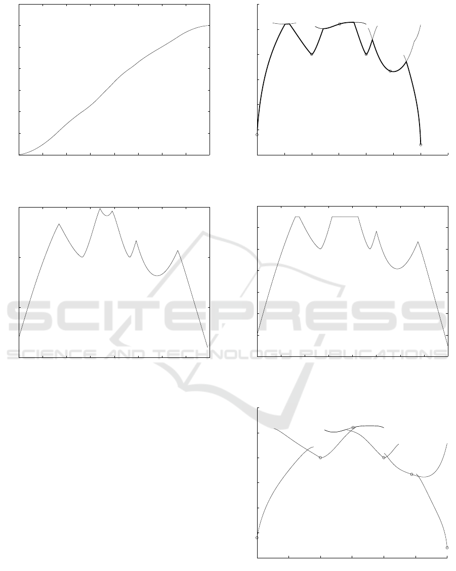
To simulate maximum driving velocity constraint
v
MAX
= 1.3m/s the resulting optimal velocity profile
changes as shown in Figs. 10- 11.
If translational acceleration is limited to a
MAXt
=
1.5m/s
2
the optimal velocity profile considering ac-
celeration and velocity constraints does not exist as
the second turn point becomes unreachable as shown
in Fig. 12.
Thereforenew feasible maximal velocity (initially
set by (18)) for the second TP need to be modified by
0 0.5 1 1.5 2 2.5 3 3.5
0
0.5
1
1.5
2
2.5
3
SP
TP
1
TP
2
TP
3
TP
4
EP
u[ ]
˙u[1/s]
Figure 10: Optimal schedule ˙u (a
MAXr
= 3m/s
2
, a
MAXt
=
4m/s
2
, v
MAX
= 1.3m/s).
0 0.2 0.4 0.6 0.8 1 1.2 1.4 1.6
0
0.2
0.4
0.6
0.8
1
1.2
1.4
t[s]
v [m/s]
Figure 11: Optimal velocity profile v(t) for a
MAXr
= 3m/s
2
,
a
MAXt
= 4m/s
2
, v
MAX
= 1.3m/s.
0 0.5 1 1.5 2 2.5 3
0
0.5
1
1.5
2
2.5
3
SP
TP
1
TP
2
TP
3
TP
4
EP
u[ ]
˙u[1/s]
Figure 12: Unreachable optimal schedule. It is not possi-
ble to arrive in the second turn point with required sched-
ule velocity ( ˙u
TP
2
= 2.6 1/s at u
TP
2
= 1.5) by acceleration
a
MAXt
= 1.5m/s
2
.
C2-continuous Path Planning by Combining Bernstein-Bézier Curves
259
0 0.5 1 1.5 2 2.5 3
0
0.5
1
1.5
2
2.5
3
SP
TP
1
TP
2
TP
3
TP
4
EP
u[ ]
˙u[1/s]
Figure 13: Optimal schedule ˙ufor a
MAXr
= 3m/s
2
, a
MAXt
=
1.5m/s
2
, v
MAX
= 1.3m/s.
0 0.2 0.4 0.6 0.8 1 1.2 1.4 1.6 1.8 2
0
0.2
0.4
0.6
0.8
1
1.2
1.4
t[s]
v [m/s]
Figure 14: Optimal velocity profile v(t) for a
MAXr
= 3m/s
2
,
a
MAXt
= 1.5m/s
2
, v
MAX
= 1.3m/s.
taking minimal off all local profiles at the u
TP
2
= 1.5
which reads ˙u
TP
2
= 2.5 1/s. The resulting optimal
profile is then feasible as shown in Figs. 13-14.
4 CONCLUSION
The use of the fifth-order Bernstein-B´ezier are pro-
posed as the path sections comprising robot path in
a hybrid path planing approaches. To obtain evenly
spread of the path section candidates in each node end
points of the sections and their orientations are pre
computed assuming constant translational and angu-
lar velocity. From those final locations together with
smooth transition requirements between the sections
the Bernstein-B´ezier polynomials aredefined. For ob-
tained composed path also an optimal velocity profile
optimization approach is illustrated. The proposed
approaches can be applied to a continuous path plan-
ing algorithm to find continuous curvature path with
no additional smoothing required. Future issues will
deal with computational complexity where velocity
profile determination is integrated in the path planing.
To obtain more optimal trajectories with shorter trav-
elling time also variable final orientation of the path
section candidates will be considered.
REFERENCES
Berglund, T., Erikson, U., Jonsson, H., Mrozek, K., and
Soderkvist, I. (2011). Automatic generation of smooth
paths bounded by polygonal chains. In Proc. of the In-
ternational Conference on Computational Intelligence
for Modelling, Control and Automation (CIMCA),
pages 528–535, Las Vegas.
Brezak, M. and Petrovi´c, I. (2014). Real-time approxima-
tion of clothoids with bounded error for path plan-
ning applications. IEEE Transactions on Robotics,
30(2):507–515.
Chen, C., He, Y., Bu, C., Han, J., , and Zhang, X. (2014).
Quartic Bezier Curve based Trajectory Generation for
Autonomous Vehicles with Curvature and Velocity
Constraints. In IEEE International Conference on
Robotics and Automation (ICRA), pages 6108–6113,
Hong Kong.
Choi, J.-W., Curry, R., and Elkaim, G. (2010). Machine
Learning and Systems Engineering, chapter Piece-
wise Bezier Curves Path Planning with Continuous
Curvature Constraint for Autonomous Driving, pages
31–45. Lecture Notes in Electrical Engineering 68.
Springer Science+Business Media.
Choset, H., Lynch, K., Hutchinson, S., Kantor, G., Burgard,
W., Kavraki, L., and Thrun, S. (2005). Principles
of robot motion: theory, algorithms, and implemen-
tations. MIT Press.
Dolgov, D., Thrun, S., Montemerlo, M., and Diebel, J.
(2008). Practical Search Techniques in Path Planning
for Autonomous Driving. pages 1–6.
Dubins, L. (1957). On curves of minimal length with a con-
straint on average curvature and with prescribed initial
and terminal positions and tangents. Amer. J. Math.,
79:497–516.
Kallmann, M. (2005). Path Planning in Triangulations. In
Proceedings of the Workshop on Reasoning, Repre-
sentation, and Learning in Computer Games, Interna-
tional Joint Conference on Artificial Intelligence (IJ-
CAI), pages 49–54, Edinburgh, Scotland.
Klanˇcar, G., Zdeˇsar, A., Blaˇziˇc, S., and
ˇ
Skrjanc, I. (2017).
Wheeled mobile robotics - From fundamentals to-
wards autonomous systems. Elsevier, Butterworth-
Heinemann.
Latombe, J.-C. (1991). Robot Motion Planning. Kluwer
Academic Publishers.
LaValle, S. M. (2006). Planning algorithms. Cambridge
University Press.
Lepetiˇc, M., Klanˇcar, G.,
ˇ
Skrjanc, I., Matko, D., and
Potoˇcnik, B. (2003). Time optimal path planning
ICINCO 2017 - 14th International Conference on Informatics in Control, Automation and Robotics
260

considering acceleration limits. Robotics and Au-
tonomous Systems, 45:199–210.
Schwartz, J. and Sharir, M. (1990). Algorithms and
Complexity, chapter Algorithmic motion planning in
robotics, pages 391–430. Elsevier.
Sencer, B., Ishizaki, K., and Shamoto, E. (2015). A cur-
vature optimal sharp corner smoothing algorithm for
high-speed feed motion generation of NC systems
along linear tool paths. Int J Adv Manuf Technol,
76(9):1977–1992.
Sethian, J. (1999). Fast Marching Methods. SIAM Review,
41(2):199–235.
Yang, X. and Wushan, C. (2015). AGV path planning based
on smoothing A* algorithm. International Journal
of Software Engineering and Applications (IJSEA),
6(5):1–8.
C2-continuous Path Planning by Combining Bernstein-Bézier Curves
261
