
Modelling Cyber Vulnerability using Epidemic Models
Bao Nguyen
Defence Research Development Canada and University of Ottawa, School of Mathematics and Statistics, Canada
Keywords: Cyber Defence, Epidemic Models, Biological Diseases, SIR (Susceptible – Infected – Removed) Model.
Abstract: This paper documents an epidemic model known as SIR (Susceptible – Infected – Removed units). We
derive an approximated solution to the differential equations that define the SIR model. Unlike the exact
SIR solution, the approximate solution is analytical and has a closed form expression. We use this
approximate model as an inspiration to cyber defence. Such a model allows us to investigate the
characteristics of the propagation of electronic viruses. That is, we can determine the number of susceptible
units, the number of infected units and the number of removed units as a function of time. This information
will eventually permit the defence to find ways to eradicate a virus attack and to show how viruses affect the
defence effectiveness.
1 INTRODUCTION
“Infectious diseases have been a part of the human
condition since time immemorial” (Smith? 2008a).
Note the “?” is part of the last name “Smith?”.
Nowadays, we also encounter electronic viruses
which can attack computers and networks. The
nature of data communication allows electronic
viruses to propagate data rates ranging from kilobits
per second to gigabits per second. Hence a network
could be infected in a matter of minutes. To prepare
defence against viruses, we need to be able to model
the process of infection. Our inspiration is owed to
the modelling of epidemiology.
“Mathematical epidemiology has its roots in
1760, when Daniel Bernoulli formulated and solved
a model for smallpox. In 1906, Hamer used a
discrete-time model of measles to understand
recurrent epidemics” (Smith? 2008b). Clearly, there
is an available body of knowledge in the
mathematics of infectious diseases.
We encounter computer viruses every day and in
every field of work. There are lots of speculations on
the potential damages of a cyber-attack. Below is a
list of examples.
a. A car’s accelerator can be disabled (Greenberg,
2016a);
b. A car can unintentionally accelerate, brake or
steer (Greenberg, 2016b);
c. A sniper rifle can be deactivated or change its
target (Greenberg 2016c);
d. The fact that North Korea’s missile launches
were failing too often may be due to US cyber-
attacks (Sanger 2017).
Some of the above examples may be real and
some of them may not be accurate. But whatever
their veracities are, cyber defence is real. It was even
mentioned in the presidential debate between Hilary
Clinton and Donald Trump (Blake 2016). It is not
hard to imagine what would happen if a defence
system is infected. The impact could range from
minor nuisances to catastrophic failures. For
example, the defence system can fire in the wrong
direction, at the wrong target and at the wrong time.
The economic impact of crimes in cyberspace is
also speculated. Below are two examples.
a. The cost of crimes in cyberspace is estimated
to be 445 billion USD (World Economic
Forum 2016) and
b. US, China and Germany, three of the four
largest economies in the world, lost more than
200 billion USD (Centre for Strategic and
International Studies 2016).
In addition to the extent of a cyber-attack, it is
common knowledge that such an attack does not
necessarily require a lot of resources as cited from
(Kesan and Hayes 2012) below:
“Cyberattacks are not resource-intensive, which
renders them even more dangerous because no
practical requirement exists to limit the attackers to
being members of organized and well-funded
sources such as a nation’s military.”
232
Nguyen, B.
Modelling Cyber Vulnerability using Epidemic Models.
DOI: 10.5220/0006401902320239
In Proceedings of the 7th International Conference on Simulation and Modeling Methodologies, Technologies and Applications (SIMULTECH 2017), pages 232-239
ISBN: 978-989-758-265-3; ISSN: 2184-2841
Copyright
c
2023 by His Majesty the King in Right of Canada as represented by the Minister of National Defence and SCITEPRESS – Science and Technology Publications, Lda. Under
CC license (CC BY-NC-ND 4.0)

This is also recognized officially by NATO as
cited from (NATO fact sheet, 2016) below:
“Cyber threats and attacks are becoming more
common, sophisticated and damaging. The Alliance
(NATO) is faced with an evolving complex threat
environment. State and non-state actors can use
cyber-attacks in the context of military operations.”
Given the frequency and extent of cyberattacks,
we investigate the infection of viruses on a network
using an epidemic model. It is certainly not the first
time that cybersecurity is modelled by epidemiology
(Krishnan et al. 2013). There are several such
models. To name a few: the SEIR model
(Susceptible-Exposed-Infectious-Recovered), the
SIR model (Susceptible-Infectious-Recovered), the
SI model (Susceptible-Infectious) and the SIS model
(Susceptible-Infectious-Susceptible) (Keeling and
Rohani 2007). Each model is named after the
sequence of phases an entity is in when infected by a
virus.
The difference between the first two, the SEIR
model and the SIR model, is that the former
simulates the exposed phase where an individual can
be infected but is not infectious. It is often possible
to remove the exposed phase from the model which
leads to the SIR model (Keeling and Rohani 2007)
where an individual can be susceptible, infected or
recovered. This can be done when the population
scale is small meaning that every individual can be
infected in a short time. Susceptible units are those
that can be infected. Infected units are those that can
infect other units. And Removed units are those that
are no longer infected (recovered units).
In contrast to the SIR model, the SI model does
not account for the recovered phase. The SI model is
usually appropriate for plants. Once the plants are
infectious, they will remain infectious and
eventually die (Keeling and Rohani 2007). The
remaining model i.e. the SIS model is appropriate
for sexually transmitted diseases. Once an individual
recovers, he/she is again susceptible to infection
(Keeling and Rohani 2007). This could be applicable
for computer viruses as well. However, for a short
time scale, we assume that the defence will not be
attacked by the same virus or that once the virus is
known; the defence will recognize its signatures and
will stop the known virus before any infections
occur.
Based on the nature of the cyber defence
scenarios that we consider: suitability of the level of
details, rapid dissemination of the infection (time
scale is short) (Hethcote 2000) and the fact that a
recovered unit is not susceptible to infection once
the virus is known and there is a software that can
neutralize the virus, we choose to examine the SIR
model as a cyber defence model.
Similar to most of the epidemic models, the SIR
model does not have an analytical solution. Hence,
it only has numerical solutions which make it
inconvenient (but not impossible) to analyze and to
predict the extent of the infection. However, we
were able to find an approximate solution that is
analytical. And we will show in future work that the
approximated SIR model is useful in planning
against cyberattacks. (Morris-King and Cam 2015)
also makes use of the SIR model to examine cyber
vulnerabilities but from an agent based simulation
perspective.
Section 2 presents the SIR model. Section 3
derives an approximated differential equation to the
SIR model. Section 4 derives an approximated
solution which is a solution to the approximated
differential equation. Section 5 analyses the results.
Section 6 provides the characteristics of the
approximated solution. We conclude in Section 7.
Before we delve into the details of the report, we
state below the assumptions:
a. It is possible for a red force to hack into the
defence system and put a virus in the defence
system;
b. The defence is partially disabled if not
completely during the infection;
c. The nature of computer viruses can be
simulated by biological epidemic models and
d. Further studies/experiments can determine the
parameters of the epidemic models.
Note that the epidemic models described above are
simple and deterministic. There are also stochastic
models (Bailey 1975) but they are even more
complicated mathematically and are not necessarily
better for our purpose than the SIR model. In fact,
there are a multitude of computer viruses such as
benevolent viruses, file infectors, macro viruses, etc.
(Horton and Seberry 1997). Each of them behaves
differently. It would be impossible to model all of
them.
We ultimately aim to determine the effects of a
cyber-attack on the effectiveness of the defence and
not the details of the infection in the sense that we
are looking for orders of magnitudes for the number
of susceptible units, the number of infected units and
the number of removed units as well as the duration
of the infection. In essence, if there is a virus in the
system and if there is a remedy to that virus and both
of them can be modelled or bound by the parameters
in the SIR model then the solution to the SIR model
can be useful to the planning of cyber defence. This
solution will enable the comparison of the efficiency
Modelling Cyber Vulnerability using Epidemic Models
233
between cyber defence software against known
viruses. Knowing the magnitudes of the duration of
the infection and the magnitudes of the number of
components that are affected will help determine the
changes in defence effectiveness. This is critical
especially against an astute enemy who could launch
a missile attack at the same time as a cyber-attack.
It is not hard to imagine how things can go wrong to
a net centric defence when the command and control
is infected even if for a short time. Key measures of
effectiveness in such a missile defence scenario will
definitely be affected and will likely show losses in
effectiveness.
2 SIR MODEL OF EPIDEMICS
The SIR model is well understood, (Smith? 2008c).
It is assumed in the SIR model that there is
homogeneous mixing within the population. This
could happen if any unit is in contact with all other
units. This interpretation can be seen when we
consider a finite population for example four units in
which one of them is infected. If the infection rate is
the same for all susceptible units then all units must
be in contact with all other units. Otherwise, by
changing the initial infected unit to another unit, we
will not have the same infection rate. This
corresponds to a complete graph (Bondy and Marty
2008) which is a graph where every node is linked to
all other nodes. In other words, this is a totally
connected network. Clearly, the spread of a virus
depends on the topology of the network (Ganesh et
al. 2005 and Chakrabarti et al. 2008). That is,
infections could occur only if an infected node is
connected to another node. Therefore, we can
consider the SIR model as the worst case scenario
i.e. an infected node can infect any other nodes. We
could also think of the SIR model as an attack at the
central node which is connected to all of the other
nodes or any susceptible unit is in contact with other
infected units in a way that each susceptible unit has
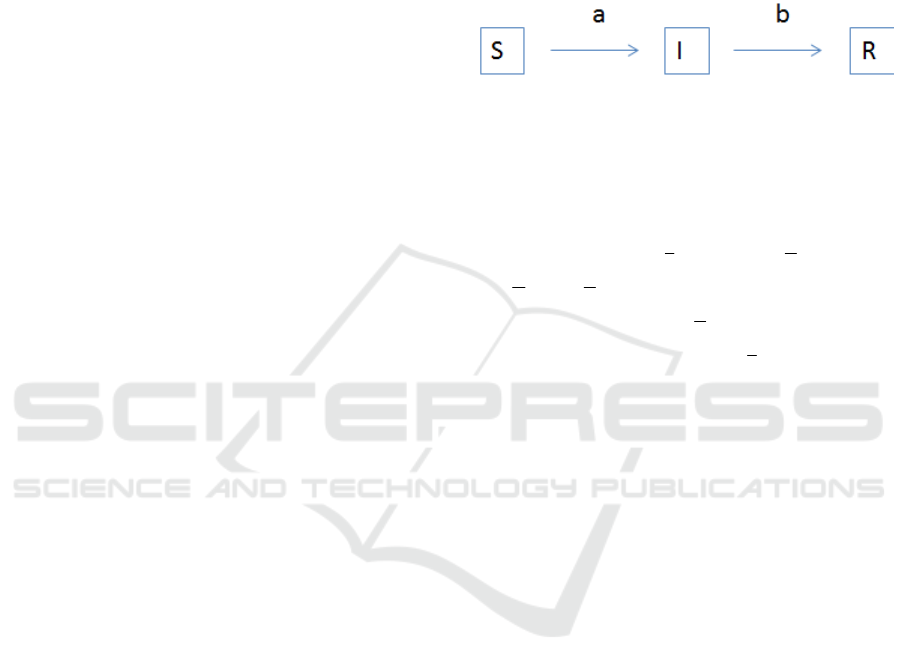
an identical rate of infection. It is defined by a set of
differential equations as shown below:
'
'
'
S aSI
I
aSI bI
RbI
=−
=−
=
(1)
where
S is the number of units that are susceptible
to infections,
I
is the number of units infected and
R is the number of units removed from infection
i.e. they are no longer infected;
a
is the rate of
infection and
b is the rate of recovery.
NSIR=++ is a constant. That is, the total
population is fixed. We scale
/, / /SSNIINandRRN←← ←. Hence,
0,, 1SIR≤≤ and 1SIR++ =. In the context of
computer viruses,
S is the number of susceptible
units,
I
is the number of infected units and R is
the number of removed (recovered) units.
Figure 1: An SIR model.
In spite of the simplicity of Equations (1), there
are no known analytical solutions. However, we
could infer from Equations (1) that there are two
equilibrium points where the RHS of Equations (1)
are equal to zeroes. The first equilibrium point
occurs when
0II==, SSN=≤ and
RRNS==−. The second equilibrium occurs
when
0aS b−=
or
/SSba== which implies
that
'0I = which makes
I
IN=≤ but S is
decreasing due to
/dS dt
. Therefore it is not a
stable equilibrium.
If
0
S is the initial value of
S
at time zero and
0
/Sba> then there will be an epidemic as
'0I >
.
The method of determining the equilibrium points
for ordinary differential equations is well
understood. It makes use of the Jacobian matrix and
its eigenvalues (Smith? 2008d). An equilibrium
point is stable if all eigenvalues are negative (or
zero).
3 APPROXIMATED
DIFFERENTIAL EQUATIONS
TO THE SIR EPIDEMIC
MODEL
We note that from Equations (1),
R
is uniquely
determined by
I
. So we focus on
S
and
I
because
once we solve for
S
and
I
, we can readily solve
for
R
. The first two equations of Equation (1) can
be combined to give:
''ISbI=− − (2)
SIMULTECH 2017 - 7th International Conference on Simulation and Modeling Methodologies, Technologies and Applications
234
We define
() ()
0
0
t
ft Itdt=≥
(3)
Integrating Equation (2), we get:
SIbfC=− − ⋅ + (4)
where
C is a constant of integration. Since
()
'/ ln 'SS S aI= =− (5)
We get
'
af
SfbfCAe
−
=− − + = (6)
where
A
is a constant parameter. If we assume that
there is
0
I
infection at time zero and there are no
removed units then these are the boundary
conditions:
() ()
()
()
0
0
0
0
00
0
00
'0
0
1
0
fItdt
fI I
SS
SI
R
==
==
=
+=
=
(7)
This means that
0
1
A
S
C
=
=
(8)
Hence,
0
'1
af
f
bf S e
−
=− −
(9)
There are two roots to the RHS of Equation (9):
/
0
1
/
0
2
11
1,
11
0,
ab
ab
aS
ff W e
ba b
aS
ff W e
ba b
−
−
−
==+ −
−
==+
(10)
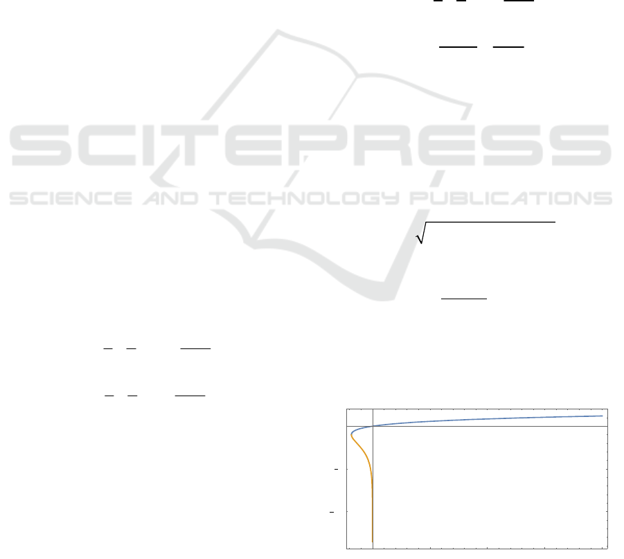
where
W is the Lambert function. The Lambert
function is shown in Figure 2. For real
x
, there are
two branches. The first branch is shown in blue and
corresponds to
()
0,Wx
while the second branch is
shown in yellow and corresponds to
()
1,Wx−
.
Since the arguments of
()
Wx
for
1
f
and
2
f
are
negative, we can infer that the
Ws
embedded in
1
f
and
2
f
are also negative based on Figure 2. Simple
calculus dictates that
00
/
u
Sue S e
−
−≥−
where
/uab=
. From Equations (1), there are two cases.
First, if
()
1abu<<
then the number of infected
units will decrease right away. That is, the infection
will die out with time. Second, if
()
1abu≥≥
then
the number of infected units will increase at least at
time zero. Therefore, we will focus on the second
case because the virus will infect the system which
is the scenario that we are interested in. Since
0
1S ≤ , we reason that:
()
0
0, 1
u
WSue
λ
−
−=−≥− (11)
Hence
/
0
2
11
0,
0
ab
aS
ff W e
ba b
abu
ab bu
λλ
−
−
==+
−−
==≥
(12)
From (Higham et al. 2015), the second order
approximation of
()
1,Wx−
is given by:
()
2
1/1
1, 1
z
We z
−−
−− =−− (13)
Equating
2
1/1
0
z
u
eSue
−− −
= (14)
We obtain:
()
0
2ln ln 1zSuu=− + −+ (15)
If
0
1S then by using a Taylor expansion, we get
()
()
()
2
3
1
11
3
u
zu Ou
−
=−+ + − (16)
As a result
()
()
2
2
1/1
1, 1 / 3
z
We uu
−−
−− −− − (17)
0 1 2 3 4
10
5
0
x
W
Lambert function
Figure 2: Lambert function.
Modelling Cyber Vulnerability using Epidemic Models
235
Hence
()
/
0
1
2
11
1,
1
0
3
ab
aS
ff W e
ba b
u
a
−
−
==+ −
−
=− <
(18)
The above holds in general for
0
01S<≤. We
observe that the RHS of Equation (9) is concave.
That is,
() ()()
1
22
xy
RHS RHS x RHS y
+
≥+
(19)
Equivalently,
()
()
()(){}
()
()
()
()
2
0
?
00
?
2
?
2
2
/2 /2
1
2
1
11
2
1
2
1
02
2
0
xy
a
ax ay
xy
a
ax ay
xy
a
ax ay
ax ay
xy
bSe
bx S e by S e
eee
ee e
ee
+
−
−−
+
−
−−
+
−
−−
−−
+
−−
≥−− +−−
−≥− +
≤− +
≤−
(20)
Because the RHS of Equation (9) is concave, we
approximate it by a quadratic function. That is,
()()
12
1
af
bfe cff ff
−
−− − −
(21)
where
1
f
and
2
f
are given by Equations (10).
Additionally, we determine
c by minimizing the
2
χ
i.e.
()()
()
2
2
12
0
min
1
f
af
c
cf f f f
df
bf e
−⋅
⋅−⋅− −
⋅
−⋅ − +
(22)
which is the same as
()()
()
()()
()
()()
2
2
2
12
0
12
12
0
1
0
1
0
f
af
o
f
af
o
cf f f f
d
df
dc
bf S e
cf f f f
df ff ff
bf S e
−
−
−−
−− − +
−−
−−=
−− − +
=
()()
()()
()
2
22
12
12
0
0
1
f
af
o
cf f f f
df ff ff
bf S e
−
−−
−− − =
−− +
(23)
This yields:
()()
()
()()
{}
2
2
12
0
22
12
0
1
f
af
o
f
ff ff
df
bf S e
c
df f f f f
−
−−
−− +
=
−−
(24)
There is actually a closed form expression for
c .
It can be obtained by performing the integrals in the
numerator and in the denominator above. However,
it is not particularly illuminating so we keep
Equation (24) the way it is. Observe that the
integrals in Equation (24) are integrated from
0f =
to
2
0ff=> since we know that
()
0ft≥ as
shown in Equation (3). By doing so, we discard all
negative values of
f
which are not physical values.
That is, the value of
c
is not affected by the value of
f
when
f
is negative.
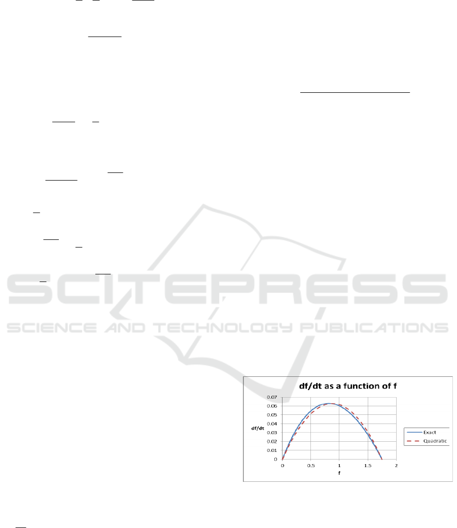
We plot the exact
/df dt
in Equation (9) and the
quadratic function in Equation (21) that
approximates
/df dt
in Figure 3. It can be seen that
the approximation is very similar to the exact
/df dt
. Both of them are concave functions with a
maximum between
1
f
and
2
f
.
Figure 3: Derivative of
f
.
For illustration, we assume the following values in
Figure 3:
0
5
12
1/ 2, 1/3
0.99999
5.99991 10 1.74847
,
ab
S
ff
−
==
=
=− ⋅ =
(25)
SIMULTECH 2017 - 7th International Conference on Simulation and Modeling Methodologies, Technologies and Applications
236
4 APPROXIMATED SOLUTION
TO THE SIR EPIDEMIC
MODEL
We now solve for
()
f
t using the quadratic
approximation:
()()
12
'
f
cf f f f−−= (26)
This is a simple differential equation that can be
solved using:
()()
12
df
dt
cf f f f
=
−−
(27)
(Gradshteyn and Ryzhik 1979) integrating:
1
2
1
ln
ff
tC
ff
−
=+
−
Δ
(28)
where
C is a constant parameter and
()
12
0cf fΔ= − > assuming that
0c <
,
1
0f <
and
2
0f > . Raising Equation (28) as a power of an
exponential, we get:
()()
12
/
t
ff f f Ae
Δ
−−=⋅ (29)
where
A
is a constant parameter. Since
()
00f =
,
this yields:
1
2
f
A
f
=−
(30)
Solving for
f :
()
2
21
1
/
t
t
fe
f
f
fe
Δ
Δ
−+
=
−+
(31)
We can now obtain
()
I
t :
() ()
()
()
2
12 1 2
2
21
'
t
t
cf f e f f
It f t
ffe
Δ
Δ
−
==
−
(32)
From Equation (5) and the boundary conditions in
Equations (7), we get an expression for
()
St:
()
()
0
af t
St Se
−
= (33)
From Equation (1) and the boundary conditions in
Equations (7), we get an expression for
()
Rt:
() ()
Rt bf t= (34)
To investigate the long term effects of the system,
we evaluate the SIR as time tends to infinity.
()
()
()
2
12 1 2
2
21
lim lim 0
t
tt
t
cf f e f f
It
ffe
Δ
→∞ →∞
Δ
−
==
−
(35)
()
()
2
21 2
1
/
00
lim lim
t
t
fe
a
f
fe af
tt
S t Se Se
Δ
Δ
−+
−
−+ −
→∞ →∞
== (36)
()
()
2
2
21
1
lim lim
/
t
t
tt
fe
Rt b bf
ffe
Δ
Δ
→∞ →∞
−+
==
−+
(37)
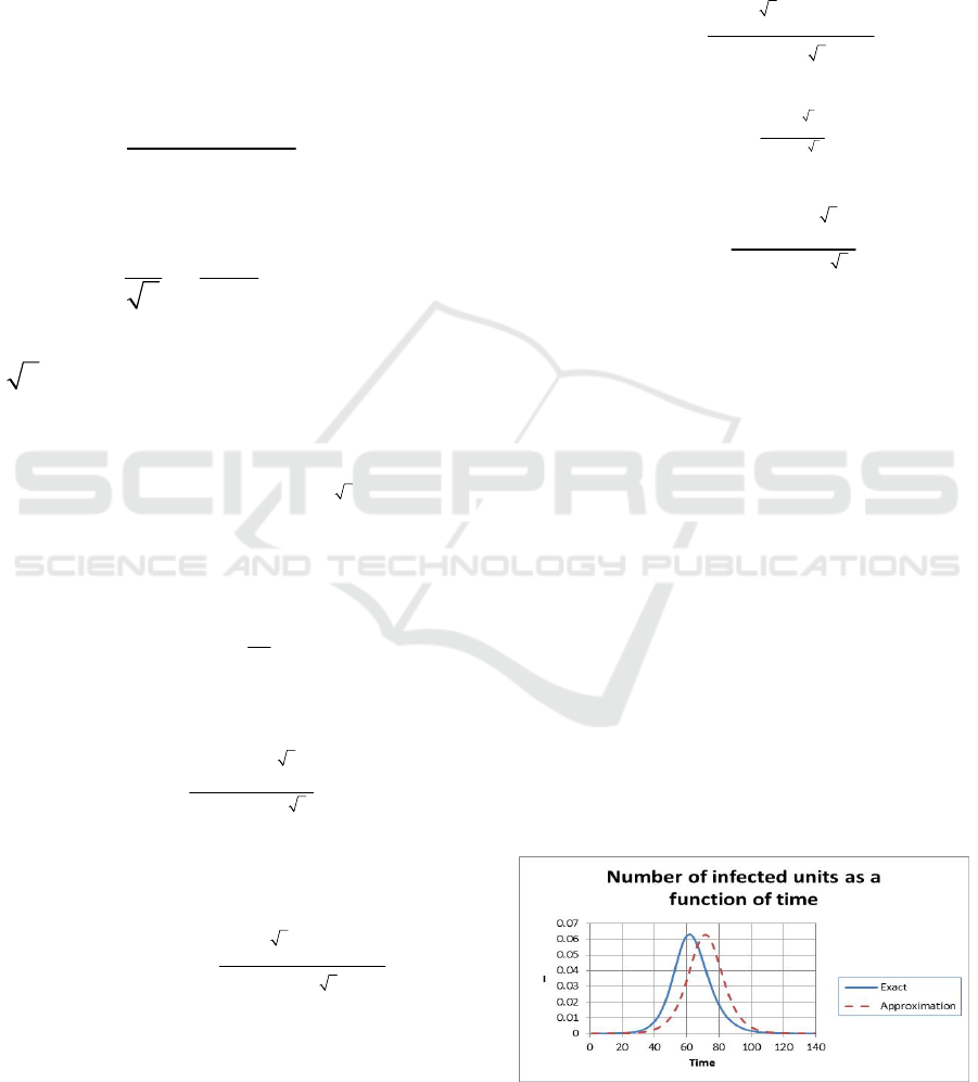
5 RESULTS
We plot
I
as a function t in Figure 4.
I
increases
as a function of time then reaches a maximum and
then decreases as a function of time. The blue curve
corresponds to the exact solution obtained
numerically while the red curve corresponds to the
approximated solution. The two have the same
shape and the same asymptotic behaviours as time
gets large. In addition, the approximated solution is
slightly shifted to the right. The maximum number
of infected units is about
6.2 percent of the
population as
I
is normalized. The input parameters
are shown in Equation (25). Note that we did not
give a unit for the time as we do not know the
coupling parameters a and
b . Once we obtain the
values for the coupling parameters, we will be able
to extract the unit of time. This will be done in the
future.
Figure 4: Number of infected units as a function of time.
Modelling Cyber Vulnerability using Epidemic Models
237
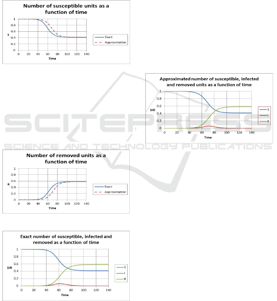
Similarly, we plot
S as a function of t in Figure 5.
It is a decreasing function of time. The blue curve
corresponds to the exact solution while the red curve
corresponds to the approximated solution. The two
have the same shape and the same asymptotic
behaviours as time gets large. That is,
S reaches a
constant value that is non-zero for large time. In
addition, the approximated solution is slightly
shifted to the right.
Figure 5: Number of susceptible units as a function of
time.
The same behaviours occur when we plot R as
a function of
t as shown in Figure 6. It is an
increasing function of time and reaches a non-zero
value as time gets large. We plot the SIR units as a
function of time for the exact model in Figure 7 and
for the approximate model in Figure 8. As time gets
large, the SIR units in both cases reach steady
values.
Figure 6: Number of removed units as a function of time.
Figure 7: Number of susceptible, infected and removed
units as a function of time.
6 CONCLUSIONS
In this paper, we have derived an approximated SIR
model and found the corresponding analytical
solution. We could consider the approximated SIR
model itself a SIR model. After all, the exact SIR
model is a man-made model where the couplings
among the susceptible units, the infected units and
the removed units are parts of the modelling.
Unlike the exact SIR model and in spite of its
simplicity, the analytical nature of the approximate
solution allows one to determine the long term
characteristics of the SIR units, the maximum
number of infected units and the time when this
occurs with only three parameters
12
,,cf f and the
boundary conditions.
12
,,cf f are obtained from the
couplings
,ab
of the exact SIR model and the
boundary conditions.
Figure 8: Number of susceptible, infected and removed
units as a function of time.
This allows us to plan for cyber-attacks.
Knowing
12
,,cf f, we can determine the extent of
the damage i.e. the number of infected units, the
number of susceptible units and the number of
removed units as functions of time. These numbers
are illustrated in Figure 4, Figure 5 and Figure 6
respectively. They show how long the system takes
to recover e.g. when the number of infected units
reaches a minimum acceptable value after attaining a
maximum value. If it takes a long time relative to
the time scale of a simultaneous missile attack then
clearly the defence may not be effective especially if
critical defence systems are infected and the defence
loses its net centric capabilities for example. What is
more, if the number of infected units keeps
increasing with time then we know that our cyber
defence is absolutely not effective. These
qualitative features and their orders of magnitudes
will be useful to the defence planning.
SIMULTECH 2017 - 7th International Conference on Simulation and Modeling Methodologies, Technologies and Applications
238

A contribution to this paper is the simplicity of
the approximated and analytical solution. We require
only the three parameters of a quadratic
function
12
,,cf fto model a generic virus infection
and its remedy.
Our next step is to conduct experiments and/or
investigations to determine these parameters that are
specific to the scenario. To do that, we would also
need to consider the number of platforms, the
number of computers, the network topology, etc.
ACKNOWLEDGEMENTS
I would like to thank Prof. Suruz Miah of Bradley
University and Dr. Kevin Ng of Defence R&D
Canada – Centre for Operational Research and
Analysis (DRDC CORA) for discussions. The
content of this paper comes from an internal
document of DRDC.
REFERENCES
Bailey, Norman T. J., 1975, The mathematical theory of
infectious diseases and its applications, Charles Griffin
& Company LTD, 2nd edition, pp. 39-42.
Blake A., The first Trump-Clinton presidential debate
transcript, the Washington Post 26 Sep 2016 (online),
https://www.washingtonpost.com/news/the-fix/wp/
2016/09/26/the-first-trump-clinton-presidential-deba
te-transcript-annotated/ (Access date: 27 Oct. 2016)
Bondy J. A. and Marty U. S. R., 2008, Graph theory.
Springer, p. 4.
Chakrabarti D., Wang Y., Wang C., Leskovec J., and
Faloutsos C., 2008. Epidemic thresholds in real
networks, Association for Computing Machinery
Transaction Information System Security. 10:4,pp.1–26.
Ganesh A., Massoulie L., and Towsley D., 2005, The
effect of network topology on the spread of epidemics,
Proceedings of IEEE Infocom.
Gradshteyn, I. S., and I. M. Ryzhik, 1979. Tables of
integrals, series, and products, 6th ed. Academic Press,
San Diego, CA. 6th Ed., p. 1100.
Greenberg, A., 2016a. Hackers remotely kill a Jeep on the
highway – with me in it, https://www.wired.com/2015/
07/hackers-remotely-kill-jeep-highway/ (Access date:
26 Oct. 2016).
Greenberg, A., 2016b. The Jeep hackers are back to prove
car hacking can get much worse, Andy Greenberg,
https://www.wired.com/2016/08/jeep-hackers-return-
high-speed-steering-acceleration-hacks/ (Access date:
26 Oct. 2016).
Greenberg, A., 2016c. Hackers can disable a sniper rifle or
change its target, Andy Greenberg, https://www.
wired.com/2015/07/hackers-can-disable-sniper-rifleor-
change-target/ (Access date: 26 Oct 2016).
Hethcote, H., 2000. The mathematics of infectious
diseases, SIAM Review, Vol. 42, No. 4, pp. 599-653.
Higham, N. J. etal, 2015. The Princeton companion to
applied mathematics, Princeton University Press, pp.
151-154.
Horton J and Seberry J, 1997, Computer Viruses: an
Introduction, Proceedings of the Twentieth
Australasian Computer Science Conference eb. 1997, -
Aust. Computer Science Communications, Vol. 19,
No. 1, pp. 122-131.
Keeling Matt J. and Rohani, P., 2007. Modeling Infectious
Diseases in Humans and Animals, Princeton
University Press, p. 4.
Kesan J, and Hayes C., 2012. Mitigative counterstriking:
self-defense and deterrence in cyberspace, Harvard
Journal of Law and Technology (forthcoming,
available at SSRN: http://ssrn.com/abstract=1805163).
Krishnan G. S. S. et al., 2013. Computational intelligence,
cybersecurity and computational models: proceedings
of ICC3, Springer.
Morris-King, J. and Cam, H., 2015. Ecology-inspired
cyber risk model for propagation of vulnerability
exploitation in tactical edge, Proceedings of the IEEE
2015 Military Communications Conference
MILCOM'2015, pp. 336-341.
Sanger, D., 2017. A Eureka moment for two times
reporters: North Korea’s missile launches were failing
too often, the New York Times, Mar 06 2017.
Smith? R., 2008a. Modelling disease ecology with
mathematics, American Institute of Mathematical
Sciences, p 1.
Smith? R., 2008b. Modelling disease ecology with
mathematics, American Institute of Mathematical
Sciences, p 1.
Smith? R., 2008c. Modelling disease ecology with
mathematics, American Institute of Mathematical
Sciences, 2008, pp. 14-16.
Smith? R., 2008d. Modelling disease ecology with
mathematics, American Institute of Mathematical
Sciences, 2008, pp. 25-30.
Xu S., Lu W., and Li H., 2015. A stochastic model of
active cyber defense dynamics, Internet Mathematics
Vol. 11, pp. 28–75.
NATO fact sheet (online), 2016. http://www.nato.int/
nato_static_fl2014/assets/pdf/pdf_2016_07/20160627
_1607-factsheet-cyber-defence-eng.pdf (Access date:
26 Oct 2016)
Net losses: estimating the global cost of cybercrime,
Centre for strategic and international studies, Jun 2014
(online), http://www.mcafee.com/ca/resources/reports/
rp-economic-impact-cybercrime2.pdf (Access date: 27
Oct. 2016).
Norton Report (online), 2013. http://www.symantec.com/
region/reg_eu/resources/virus_cost.html (Access date:
26 Oct. 2016).
The global risks report 2016, 11th edition, World
Economic Forum (online), http://reports.weforum.org/
global-risks-2016/executive-summary/ (Access date:
26 Oct. 2016).
Modelling Cyber Vulnerability using Epidemic Models
239
