Fault Detection for Heating Systems

using Tensor Decompositions of Multi-linear Models

Erik Sewe

, Georg Pangalos

and Gerwald Lichtenberg

PLENUM Ingenieurgesellschaft f

ur Planung Energie Umwelt mbH, Hamburg, Germany

Fraunhofer Institute for Silicon Technology ISIT, Application Center Power Electronics for Renewable Energy Systems,

Hamburg, Germany

Hamburg University of Applied Sciences, Faculty of Life Sciences, Hamburg, Germany

Keywords:

Fault Detection, Boilers, Heating Systems, Multi-linear System, Tensor Representation.

Abstract:

A model-based fault detection method for heating systems is proposed. Two examples of heating system units

are under investigation. These systems can be represented as multi-linear systems. Subspace identiﬁcation

methods are used to identify linear time-invariant models for each operating regime, resulting in a parameter

tensor. In case of missing data and models for some operating regimes, an approximation method is proposed,

where the canonical polyadic tensor decomposition method is used. Low rank approximations are found using

an algorithm specialized for incomplete tensors. The tensor of these approximations deﬁnes the models in

operating regimes, where no measurements were available. Fault detection is done using parity equations and

application examples using real measurement data of a heat generation unit are given.

1 INTRODUCTION

The analysis of the operation of complex heating sys-

tems usually shows potential for optimization, see

(Rehault et al., 2013). In many cases failed com-

ponents, insufﬁciently tuned controller parameters as

well as user intervention result in problems of heat

supply and excess consumption. A frequently occur-

ring problem - this shows an investigation of a mul-

titude of malfunctions of heating systems done by

PLENUM - are operation errors of combined heat

and power plants and gas boilers. This includes

faults from manipulated parameters up to complete

loss of the heat production. For this reason a con-

tinuous fault detection is desirable. Currently this

is done on a simple level, meaning threshold value

checks and ordinary rules. This is quite simple, but

reaches its limits of transferability and expandability,

see (Venkatasubramanian et al., 2003). The methods

of fault detection used for heating systems are not best

practice according to today’s technical knowledge and

options, (Katipamula and Brambley, 2005).

A model-based fault detection can provide an en-

hanced detection performance, but is associated with

many obstacles, see (Jagpal, 2006). The behavior of

heating systems and buildings is difﬁcult to predict.

Systems are unique and the creation of exact mod-

els is difﬁcult, time consuming and therefore expen-

sive. Detailed building plans and schemes are rarely

available, the intended function often poorly docu-

mented. Measurement data is intermittent or of poor

quality. Some variables are not directly measurable.

A high number of disturbances occurs. Additionally,

(sub-)system are nonlinear.

The basis of model-based fault detection is a

model of the system, that captures the main system

dynamics in a precision, that is sufﬁcient for the task.

Models of heating systems can be derived by deﬁn-

ing heat power balances, see (Pangalos, 2015). The

heat power balances have a multilinear property, aris-

ing from the multiplication of temperature spread and

ﬂow rate. Since both - temperature spread and ﬂow

rate - are states of the system or linearly depending

on a state of the system (depending on the realiza-

tion of the model) a direct description as a linear state

space model is not possible. Furthermore, discrete

signals like boiler switching (on/off) turn the prob-

lem into a hybrid one. One possibility to model these

hybrid heating systems is to use tensor systems, see

e.g. (Lichtenberg, 2011; Pangalos et al., 2015). This

approach is quite new, such that so far no methods

for system identiﬁcation exist, only standard nonlin-

ear parameter identiﬁcation algorithms - which do not

take care of the multilinear structure - could be ap-

Sewe, E., Pangalos, G. and Lichtenberg, G.

Fault Detection for Heating Systems using Tensor Decompositions of Multi-linear Models.

DOI: 10.5220/0006401400270035

In Proceedings of the 7th International Conference on Simulation and Modeling Methodologies, Technologies and Applications (SIMULTECH 2017), pages 27-35

ISBN: 978-989-758-265-3

plied. For that reason a different approach is used

here to model the system. The model of the chosen

approach could be represented as a switched system,

see (Liberzon, 2003). By quantizing one of the sig-

nals - temperature spread or ﬂow rate - no multipli-

cation of these signals is needed, because for each

quantized system the signal which was not quantized

is multiplied with a constant. Depending on the size

of the quantization interval, inaccuracies between the

original and the quantized system arise. For each in-

terval of the quantized signal and for each combina-

tion of the discrete signals one linear model is es-

timated using standard techniques, e.g. the N4SID

algorithm, (Van Overschee and De Moor, 2012), re-

sulting in several linear time-invariant systems, i.e.

a multi-linear time-invariant model. Note, that

multi-linear is used to denote multiple linear mod-

els, whereas multilinear - without dash - is used to

denote models where the multiplication of all states

and inputs - and all combinations with all numbers

of multiplicants - are admissible. In multilinear sys-

tems no square terms are allowed, this could be mod-

eled by polynomial models. Note that for polyno-

mial systems black box identiﬁcation methods exist,

see (Mulders et al., 2009). The heating systems un-

der investigation have the aforementioned multilin-

ear property that could be modeled in the polynomial

framework but the hybrid property (the discrete sig-

nals) are beyond the scope. In addition, the identi-

ﬁcation is, opposed to the one step identiﬁcation of

N4SID an iterative identiﬁcation which also needs to

be initialized, (Paduart et al., 2010).

This paper shows how this approach can be used

for fault detection in heating systems. In section 2

method and structure for estimating the parameter sets

and fault detection are explained. The complete sys-

tem can be stored in a tensor structure, see section 2.1.

Identiﬁcation of parameter sets is explained in sec-

tion 2.2. Missing parameter sets for operating points

not included in training data can be estimated by ten-

sor completion, see section 2.3. Fault detection is

done using parity equations, section 2.4. In section 3

two application examples are given. In section 4 con-

clusions are drawn.

2 MODEL-BASED FAULT

DETECTION METHOD FOR

HEATING SYSTEMS

As mentioned before heating systems can be mod-

eled as hybrid multilinear systems. Keeping all

but one signals constant in multilinear terms and

regarding just one combination of the binary sig-

nals will result in a linear behavior. Thus for

each combination of quantized and binary signals,

which will be denoted as operating regime, see

(Murray-Smith and Johansen, 1997), a linear system

can be identiﬁed around an operating point. For each

operating regime, measurement data is used to iden-

tify a model. If a large amount of data is available

for one operating regime, the measurement data is

divided into parts, which will be called operational

sections. The set of linear systems for all operating

regimes will be denoted as parameter tensor.

2.1 System Deﬁnition

The operating regime I is deﬁned by the combination

of binary signals (e.g. on/off, opened/closed) and the

center of the intervals of quantized signals (e.g. tem-

peratures, ﬂow rates). The signals will be denoted as

partitioning signals, v is the number of partitioning

signals. The operating regime is deﬁned by the index

vector

I = (i

, i

, . . . , i

) (1)

with i

= {1, 2, . . . , I

}, n = 1, 2, . . . , v. The

number of partitions of the corresponding signal

is I

, n = 1, 2, . . . , v. Note that I

= 2 for all binary

signals, it is assumed that 0 corresponds to index 1

and 1 corresponds to index 2. For the continuous-

valued operating regime deﬁning signals, the inter-

vals J

, . . . , J

are used for quantization. The index of

these intervals is also the corresponding index in the

index vector I. The limits of the intervals are stored.

As an example, for a system with one continuous-

valued operating regime deﬁning signal divided into

ﬁve sections and one binary signal, the index vector

is I = (i

, i

) with i

∈ {1, . . . , 5} and i

∈ {1, 2}.

Around each operating regime a linearization is per-

formed. The result of the linearization is a discrete-

time state space model

x(k +1) = A

x(k) +B

u(k) (2)

y(k) = C

x(k) +D

u(k) (3)

where k denotes the time index, I the mode of oper-

ation, x ∈ R

the state vector, u ∈ R

the input vec-

tor, y ∈ R

the output vector, A

∈ R

n×n

the system

matrix, B

∈ R

n×m

the input matrix, C

∈ R

p×n

the

output matrix and D

∈ R

p×m

the feed forward ma-

trix. Please note that the A, B, C, and D matrices

must be in a canonical state space representation. The

representation as given in (4) is used to store the en-

tire information of the state space model in a single

matrix, that has dimension R

(n+p)×(n+m)

. Also given

in (4) are the elements of A, B, C, and D in state space

SIMULTECH 2017 - 7th International Conference on Simulation and Modeling Methodologies, Technologies and Applications

modal representation. The systems do not have a di-

rect feedthrough, so D is a zero matrix.



A B

C D









0 . . . 0 b

. . . . . . b

0 a

0 . . . 0 a

. . . . . . b

. . . . . . c

0 . . . . . . 0

. . . . . . c

0 . . . . . . 0







(4)

To represent the entire multi-linear system, i.e. a lin-

ear system for each combination of the v signals,

deﬁning the operating regime, the parameter tensor M

M ∈ R

(n+p)×(n+m)×I

×I

×···×I

(5)

is created, where the notation of

(Cichocki et al., 2009) is adapted. The entries

of the third to the v

+ 2 dimension of M correspond

to the operating regime I. Keeping all but the ﬁrst

two dimensions constant will give the



A B

C D



matrix of the linear system that is identiﬁed for

operating regime I. This matrix is selected despite

the amount of zeros in A and D, to allow a generic

system description. The linearization is performed

for speciﬁc values of the input and output signals.

Recall that so far the operating regime was denoted

as a point deﬁning a linear system, i.e. basically the

switching signal if a switched afﬁne system would

have been used. But to ﬁnd a good approximation

also the inputs and outputs of the linear systems need

to be at their operating point. These values also need

to be stored, but for reasons of size and magnitude

they do not ﬁt into M. The input and output operating

point values

and

are stored in the additional

tensor O

O ∈ R

(m+p)×I

×I

×···×I

(6)

with

O(:, I) = [

]

. (7)

2.2 Identify Parameter Tensor Slices

The ﬁrst step is to read input and output data as well

as signals that determine the operating regime. De-

pending on the data quality some pre-processing such

as outlier removal and ﬁlling data gaps must be done.

By quantization the values of the partitioning signals

are partitioned into intervals. The interval edges are

stored and used for quantization of the application

data. The next step is to detect operating regimes

and sort data by operating regimes. For each oper-

ating regime the operating point for input and out-

put data is stored in O. For black box estimation

of the state-space matrices, MATLAB provides the

N4SID algorithm in the System Identiﬁcation Tool-

box (Ljung, 2016). A noise component is not esti-

mated, the value is ﬁxed to zero. The MATLAB com-

mand canon with option modal transforms a linear

model into a canonical state-space model in modal

representation. As it does not normalize the B or C

matrix this is done by normalizing the non-zero en-

tries of C for the ﬁrst output to f

. Tensor algorithms

are sensitive to scale of data elements (Fanaee-T and

Gama, 2016), so the parameter f

should be chosen

in a way that all resulting entries have the same scale.

The transformation is performed as in (8) to (12).

norm

= f







0 . . . 0

. . . 0

0 0 . . .







(8)

norm

= T

−1

norm

(9)

norm

= T

−1

norm

B (10)

norm

= CT

norm

(11)

norm

= D (12)

For better readability, in this paper it is assumed that

the matrices A, B, C, and D stored in and restored

from the parameter tensor are normalized without

stating the indices

norm

2.3 Construct Full Parameter Tensor

For systems where several binary or quantized sig-

nals are determining the operating regime, it is very

likely for some operating regimes that no measure-

ments are taken. Therefore the tensors (5) and (6) can

have unknown entries. In ﬁgure 1 a schematic view

of an incomplete parameter tensor with one partition-

ing signal is shown. To cope with this problem a ten-

unknown

measured

Figure 1: Incomplete parameter tensor, v = 1.

Fault Detection for Heating Systems using Tensor Decompositions of Multi-linear Models

sor decomposition approach is chosen. It is assumed,

that the operating regimes are not independent of each

other but that the system dynamics is inﬂuenced by

changing one speciﬁc signal which is deﬁning the op-

erating regime. The change of one signal will have

a similar effect for all operating regimes, or at least

can be reconstructed by looking at the change of all

operating regime components. To ﬁll up the miss-

ing entries in the tensors M and O the tensorlab tool-

box, (Vervliet et al., 2016), for MATLAB is used. It

is assumed, that if a low rank approximation is found,

which can represent the existing entries of the ten-

sors, the system dynamics of all operating regimes

are contained in this tensor. By resolving the entire

tensor entries for the previously not deﬁned operat-

ing regimes can be found. To decompose the tensor

the canonical polyadic decomposition algorithm cpd

of the tensorlab toolbox is used. All entries of the ten-

sor, which are unknown, are deﬁned as non existing,

which is done by setting the corresponding entries to

the value NaN in MATLAB. The used algorithm op-

tion CPDI is set to true such that a routine is used,

which is specialized to cope with incomplete tensors.

The general idea to ﬁnd a decomposed tensor, i.e. the

factor matrices F

for a tensor T is to solve the mini-

mization problem

min

(1)

,...,F

(H)



T −

(1)

, . . . , F

(H)



(13)

where F

(1)

, . . . , F

(H)

denote the factor matrices of the

decomposed tensor, [[. . . ]] is used to represent a tensor

using factor matrices and ||. . . || denotes the Frobe-

nius norm, (Vervliet et al., 2014). The specialized

routine solves the problem

min

(1)

,...,F

(H)



G ~



T −

(1)

, . . . , F

(H)

ii



(14)

where G ∈ R

×I

×···×I

is a binary observation

tensor with the entries set to 1 if the corre-

sponding value in T is known and 0 otherwise

and ~ denotes the Hadamard, i.e. the element-wise

product (Vervliet et al., 2014). Solving this mini-

mization problem does not take into account any un-

known values.

Obviously this approach can just be used if for a

sufﬁciently large number of operating regimes a lin-

ear state space model can be identiﬁed. If the entire

system dynamic is not captured by the measured op-

erating regimes, resolving the tensor will not yield

in a good approximation for the unmeasured oper-

ating regimes. Note also that the selection of the

rank of the approximation is not trivial. Increasing

the rank will introduce freedom in choosing the val-

ues of the unidentiﬁed tensor entries and thus not re-

sult in a good approximation, choosing a rank which

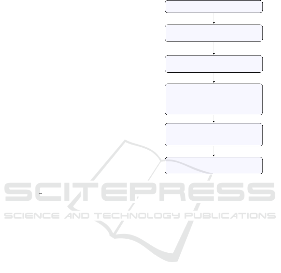
Read and preprocess data

Detect operating regimes and

divide data into operational sections

Merge data of same

operating regimes

Identify normalized canonical

state space models and operat-

ing points for each operating

regime included in the data

Save parameter matrices

and operating points in ten-

sor structures M and O.

Construct full parameter tensor

by cp tensor decomposition

Figure 2: Generating parameter tensor.

is too small results in a tensor which does not cap-

ture the system dynamics. In this paper the rank is

chosen heuristically. Choosing a high rank results in

good approximations for the known parameters in the

parameter tensor. The rank is then reduced until the

unknown parameters are the approximately same for

different initial values in the tensor decomposition.

Summing up sections 2.1 to 2.3, the parameter ten-

sor, describing the system behavior in every operating

regime, can be created as shown in ﬁgure 2.

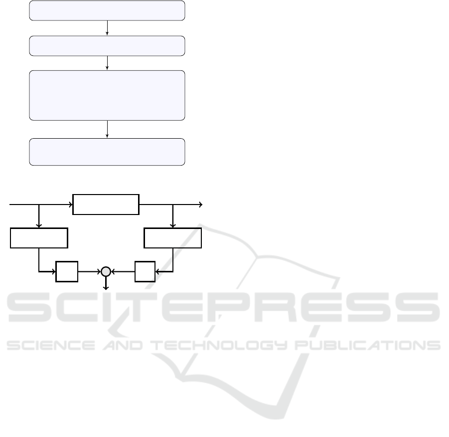
2.4 Fault Detection with Parity

Equations

The proposed method is used for ofﬂine fault detec-

tion, using parity equations. See ﬁgure 3 for the

fault detection procedure. The parameter tensor in-

troduced in section 2.1 describes the nominal, i.e. the

non-faulty behavior. Parity equations and observer

based designs are a way to detect discrepancies be-

tween process and model. Once the design objectives

have been selected, both lead to identical or equiva-

lent residual generators (Gertler, 1991). The proce-

dure for parity equations is usually simpler than for

observer based designs (Gertler, 1991). One beneﬁt

of parity equation is, that no initial value for the state

vector x is needed. Input and output data are com-

SIMULTECH 2017 - 7th International Conference on Simulation and Modeling Methodologies, Technologies and Applications

Read and preprocess data

Detect operating regimes

For each operational section

select corresponding matri-

ces A, B, C, and D from M

and operating points from O

Fault detection with parity equation

for each operational section

Figure 3: Fault detection.

heating system

tapped delay tapped delay

r(k)

−

Figure 4: Parity equation.

pared to the model behaviour contained in w and Q,

as seen in ﬁgure 4. The tapped delay block delays

the input u respectively the output y by q + 1 time

steps and outputs all the delayed versions, resulting

in U (15) and Y (16).

U(k) =







u(k −q)

u(k −q + 1)

u(k −q + 2)

u(k)







(15)

Y(k) =







y(k −q)

y(k −q + 1)

y(k −q + 2)

y(k)







(16)

The residual r at time k for q + 1 time steps is calcu-

lated by

r(k) = w

Y(k) −w

(q)U(k) (17)

with

(q) =







q−1

q−2

q−3

. . .







(18)

The derivation for (17) is explained in (Isermann,

2006). The residual generator vector w

is determined

by solving

= 0 (19)

with

(q) =













. (20)

There is more than one solution for (19). The trivial

solution must not be chosen. By selecting w

proper-

ties of fault detection are affected. The fault signal e,

where 0 stands for ’no fault’ and 1 for ’fault’ is calcu-

lated by the fault criterion

e(k) =



0 if r(k) ∈ [b

, b

]

1 else

. (21)

For every operating section the residual r(k) is com-

pared to upper and lower bound, b

and b

for the de-

cision if there is a fault or not. Due to computation

time and memory use the length of a operating sec-

tion is limited to q + 1 time steps. Operating sections

longer than q + 1 time steps are divided and exam-

ined individually. Upper bound b

and lower bound b

are determined by calculating the residual r(k) for the

data used to create M and are the same for every op-

erating regime I. This gives the decision boundary

for non-faulty operation. Values of r(k) exceeding the

range limited by b

and b

are expected to imply faulty

operation.

3 APPLICATION TO HEATING

SYSTEM FAULT DETECTION

The heat generation unit of the heating system of

the State Ofﬁce for Nature, Environment and Con-

sumerism in D

usseldorf, Germany is investigated.

The heat generation unit consists of three hydrauli-

cally balanced boilers with attached gas burners, two

Fault Detection for Heating Systems using Tensor Decompositions of Multi-linear Models

of them are condensing boilers, one is a low tem-

perature boiler. The three boilers together have a

total power of about 1870 kW and supply six con-

sumer circuits. The consumer circuits are not inves-

tigated in this paper and therefore no model of them

is given. The heating system was already under in-

vestigation in (Sewe et al., 2012; Pangalos and Licht-

enberg, 2012), where a model of the entire system is

given and the controller design and implementation

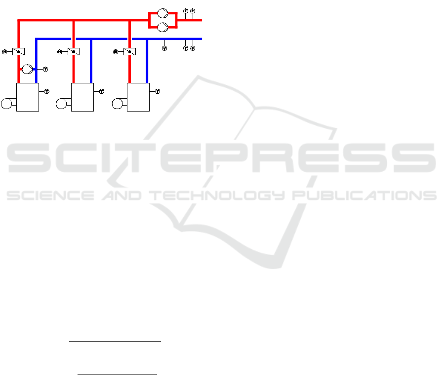
is described. A scheme of the heat generation unit

is given in ﬁgure 5. Each boiler is equipped with a

lid such that the ﬂow rate through the boiler can be

stopped when the boiler is switched off.

Boiler 1Boiler 2Boiler 3

Figure 5: Scheme of the heat generation unit.

The inputs of the model of the heat generation unit

are the return temperature T

and the power to be pro-

duced by the boilers P

, i = 1, 2, 3. The output is the

supply temperature T

. The states of the heat genera-

tion model are the supply temperatures of the boilers.

The operating regime of the heat generation unit is

deﬁned by position of the boilers lids (opened/closed)

and the burners switching signals (on/off). The ﬂow

rate is divided in four intervals. For each of these in-

tervals and each of the boiler lid and burner switching

setting, a model of the system is estimated. Result-

ing in a tensor M of dimension R

4×7×4×2×2×2×2×2×2

the operating regime index is I = (i

, i

)

with i

∈ {1, . . . , 4} and i

∈ {1, 2} for n = 2, . . . , 7.

The heat generation unit can be modelled, with some

simpliﬁcations, as described in (Kruppa, 2014) by

+ T

, (22)

+ c

− T

)

ρV

(23)

and

V =

, (24)

where T

is the supply temperature of the heat gener-

ation unit, T

is the return temperature,

V is the ﬂow

rate out of the heat generation unit and back into it, T

are the supply temperatures, V

the volumes, P

the

input powers of the boilers 1, 2 and 3 respectively,

for i = 1, 2, 3,

are the ﬂow rates through the boil-

ers, c

is the speciﬁc heat capacity of water and ρ the

water density.

3.1 Fault Detection on a Multi-boiler

System

As stated in section 2.3, tensor completion of the pa-

rameter tensor only yields in correct approximations

if a sufﬁciently large number of operating regimes

can be identiﬁed. For that reason this ﬁrst example

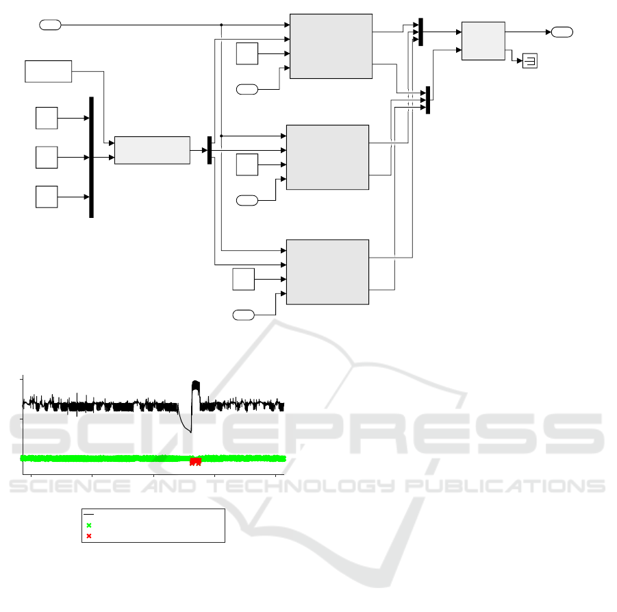
demonstrates the proposed method using a MATLAB

SIMULINK model as shown in ﬁgure 6. The model

is created with slightly simpliﬁed components of the

HeatLib (Kruppa, 2014). Its parameters are adapted

to ﬁt the heat generation unit described above.

Instead of using the N4SID algorithm, a discrete-

time linear state-space model around the operating

point is extracted, using MATLAB SIMULINK . A

complete parameter tensor is created and can be ma-

nipulated by deleting several operating regimes. Us-

ing the introduced tensor decomposition and recon-

struction method, the parameter tensor is completed

again. In (25) and (26) the A matrix for one operating

regime I is shown, where (25) is the original and (26)

the restored matrix.





0.8532 0 0

0 0.8157 0

0 0 0.7731





(25)





0.8532 −0.001 −0.000

−0.001 0.8156 −0.000

−0.001 −0.001 0.7730





(26)

The incomplete parameter tensor has stored sufﬁ-

cient information of the entire system dynamic so

that resolving the tensor yields to a good approx-

imation. The tensors M and O are used for fault

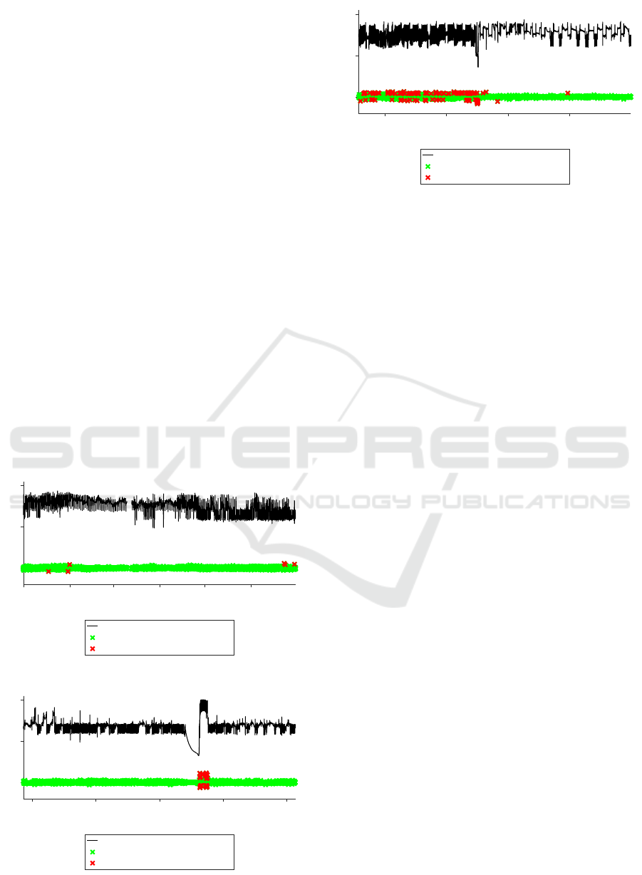
detection on real input and output data. Figure 7

shows the measured supply temperature and the re-

sulting residual r(k) for each operational section. In

case of of fault, i.e. e(k) = 1, r(k) is marked red,

for non-faulty sections it is marked green. One sum-

mer month is tested. After a complete system break-

down on June 18

the supply temperature drops to

temperatures below 35

◦

C. No fault is detected be-

cause input data is consistent to output data, boilers

are not turned on in this period. As a consequence,

on June 20

, boiler 2 has been turned on in manual

mode. It is working on full power and ignoring con-

troller signals, thus heating up the system until it is

stopped by an emergency switch, now working as a

two point controller. This does not match to expected

system behavior. The fault is detected correctly. On

SIMULTECH 2017 - 7th International Conference on Simulation and Modeling Methodologies, Technologies and Applications

[T]

[dV]

T_Vl

dV_Vl

flow rate collector

Vdot

Klappe

Vdot Kessel

flow rate distribution

supply temperature

T_Rl

dV_ein

Kessel an/aus

Modulation

T_Kessel

dV_Kessel

boiler 3

T_Rl

dV_ein

Kessel an/aus

Modulation

T_Kessel

dV_Kessel

boiler 2

T_Rl

dV_ein

Kessel an/aus

Modulation

T_Kessel

dV_Kessel

boiler 1

power 2

return temperature

power 3

power 1

Kl1

lid 1

Kl2

lid 2

Kl3

lid 3

burner 3

burner 2

burner 1

Vdot

flow rate

Figure 6: Heat generation unit modelled in SIMULINK .

06/02 06/09 06/16 06/23 06/30

day

100

measured supply temperature [°C]

r(k)

r(k) for e(k)==1

Figure 7: Fault detection - heat generation unit.

June 21

the boiler has been set back to normal oper-

ating mode.

3.2 Fault Detection on a Single Boiler

The method explained in chapter 2 is performed

on boiler 2, using black box identiﬁcation (N4SID,

MATLAB System Identiﬁcation Toolbox) to estimate

the state space matrices. It is a ﬁrst order system.

The inputs of the model of boiler 2 are the return

temperature T

and the power to be produced by the

boiler P

. The output is the supply temperature T

The state is also the supply temperature of the boiler.

The operating regime of the boiler is deﬁned by the

burner switching signal (on/off) and the ﬂow rate. As

boiler 2 is the main supplier of the heating system,

no training data with the lid closed is available and

therefore it cannot be used as an operating regime.

The ﬂow rate is divided in seven intervals. For each

of these intervals and each of the burner’s switching

setting a model of the system is estimated. Result-

ing in a tensor M of dimension R

2×3×7×2

, the oper-

ating regime index is I

= (i

, i

) with i

∈ {1, . . . , 7}

and i

∈ {1, 2}. The parameter tensor is created with

measurement data of six month. Thirteen of fourteen

operating regimes appear in this data set. For im-

proved illustration of the proposed method, parame-

ters of two known operating regimes are deleted. The

entries of the parameter tensor corresponding to the A

matrices - which are scalars in this case, since a ﬁrst

order system is under investigation - in the different

operating regimes are shown in (27), where ∗ marks

the missing modes. The seven entries in the ﬁrst di-

mension correspond to the seven intervals of the ﬂow

rate and the two entries in the second dimension cor-

respond to the burner switching signal.

M(1, 1, :, :) =







1.00 0.89

0.81 0.76

0.82 ∗

0.68 0.75

∗ 0.69

0.57 0.64

∗ 0.62







(27)

As the system can be described by (23), for all op-

erating regimes including the missing ones, it can be

assumed, that C = 1 and D = [0 0 ]. To ﬁll up the

missing entries a tensor decomposition of rank 2 is

approximated. Unfolding this tensor to a full tensor

Fault Detection for Heating Systems using Tensor Decompositions of Multi-linear Models

gives the result

M(1, 1, :, :) =







1.00 0.88

0.80 0.77

0.82 0.79

0.70 0.73

0.63 0.69

0.57 0.64

0.50 0.62







. (28)

The parameter tensor partially shown in (28) is vali-

dated on the six month of training data, see ﬁgure 8.

The six errors detected in the training data are in op-

erational sections where the lid of boiler 3 has been

opened or closed. So it is assumed, that the ﬂow

rate

, calculated by the ﬂow rate

V , hydraulic pa-

rameters and the position of the boilers lids, in these

sections is faulty due to inaccuracy in data logging.

The parameter tensor is tested on data of the same pe-

riod as used for the simulation in ﬁgure 7. As can

be seen in ﬁgure 9, the fault is detected correctly.

Another fault can be observed in a winter month as

seen in ﬁgure 10. Till December 14

, boiler 2 is

not processing the controller power signal, thus not

producing the correct amount of heat, but the burner

switching signal (on/off) is conﬁgured correctly. So

the boiler is turned on at the correct periods but does

not vary the power output. As a result, the supply tem-

perature T

exceeds the set point temperature and the

01/01 02/01 03/01 04/01 05/01 06/01

day

100

measured supply temperature [°C]

r(k)

r(k) for e(k)==1

Figure 8: Fault detection boiler 2, model validation.

06/02 06/09 06/16 06/23 06/30

day

100

measured supply temperature [°C]

r(k)

r(k) for e(k)==1

Figure 9: Fault detection boiler 2, manual operation.

12/04 12/11 12/18 12/25

day

100

measured supply temperature [°C]

r(k)

r(k) for e(k)==1

Figure 10: Fault detection boiler 2, failure in power control.

controller can not keep the multi-boiler system stable.

On December 14

, a service engineer adjusted the

parameters of boiler 2 and for the remaining time of

the data set the system worked as expected. For the

faulty part of the data set the residual r(k) has values

exceeding the range limited by b

and b

, so the fault

is detected correctly. The two errors detected after

December 15

are in operational sections where the

lid of boiler 3 has been opened or closed, so as well

as in ﬁgure 8, faulty input data for calculation of

is assumed.

4 CONCLUSIONS

A method to detect faults in heating systems has been

proposed. The fault detection is model-based such

that models of heating systems were investigated. A

multi-linear time-invariant system is constructed by

identifying multiple linear time-invariant systems for

different operating regimes. To deﬁne the operat-

ing regime, signals, which are multiplied with inputs

or states, are quantized. This multiplication arises

from the heat power balances, which are the basis

of the models. There the multiplication of tempera-

ture (which is a state) and ﬂow rate (which is an in-

put) makes the system nonlinear. By quantizing the

ﬂow rate, multiple linear systems can be deﬁned. Fur-

thermore, different binary signals extend the operat-

ing regime. For each interval of the ﬂow rate and

each binary signal, a linear system is identiﬁed. All

these systems build the parameter tensor. If for some

operating regimes no measurement data is available,

an approximation method is proposed. By estimating

low rank approximations of the parameter tensor with

specialized algorithms for incomplete tensors, good

approximations of the systems, where no measure-

ment data was available could be found. The general

functionality is shown in two application examples.

The fault in the measurement data was identiﬁed in

SIMULTECH 2017 - 7th International Conference on Simulation and Modeling Methodologies, Technologies and Applications

both examples. Work will be continued on improved

estimation of system matrices on operating regimes

with missing measurement data.

ACKNOWLEDGEMENTS

This work was partly supported by the project

OBSERVE of the Federal Ministry for Economic Af-

fairs and Energy, Germany (Grant-No.: 03ET1225C)

and partly supported by the Free and Hanseatic City

of Hamburg (Hamburg City Parliament publication

20/11568).

REFERENCES

Cichocki, A., Zdunek, R., Phan, A., and Amari, S. (2009).

Nonnegative matrix and tensor factorizations. Wiley,

Chichester.

Fanaee-T, H. and Gama, J. (2016). Tensor-based anomaly

detection: An interdisciplinary survey. Knowledge-

Based Systems, 98:130–147.

Gertler, J. (1991). Analytical redundancy methods in fault

detection and isolation. In Preprints of IFAC/IMACS

Symposium on Fault Detection, Supervision and

Safety for Technical Processes SAFEPROCESS91,

pages 9–21.

Isermann, R. (2006). Fault-diagnosis systems: an introduc-

tion from fault detection to fault tolerance. Springer

Science & Business Media.

Jagpal, R. (2006). EBC Annex 34 - computer aided eval-

uation of HVAC system performance - technical syn-

thesis report: Computer aided evaluation of HVAC

system performance.

Katipamula, S. and Brambley, M. (2005). Methods for

fault detection, diagnostics, and prognostics for build-

ing systems - a review, part I. HVAC&R Research,

11(1):3–25.

Kruppa, K. (2014). Dokumentation Matlab Heatlib - Zur

Verwendung mit Matlab. Dokumentation, Institut f

Regelungstechnik, TU Hamburg-Harburg.

Liberzon, D. (2003). Switching in systems and control,

ser. Systems & Control: Foundations & Applications.

Boston: Birkh

auser.

Lichtenberg, G. (2011). Hybrid Tensor Systems. Habilita-

tion, Hamburg University of Technology.

Ljung, L. (2016). System identiﬁcation toolbox: user’s

guide.

Mulders, A. V., Schoukens, J., Volckaert, M., and Diehl,

M. (2009). Two nonlinear optimization methods for

black box identiﬁcation compared. IFAC Proceedings

Volumes, 42(10):1086 – 1091.

Murray-Smith, R. and Johansen, T. A. (1997). Multiple

Model Approaches to Modelling and Control. Taylor

and Francis, London.

Paduart, J., Lauwers, L., Swevers, J., Smolders, K.,

Schoukens, J., and Pintelon, R. (2010). Identiﬁcation

of nonlinear systems using polynomial nonlinear state

space models. Automatica, 46(4):647 – 656.

Pangalos, G. (2015). Model-based Controller Design Meth-

ods for Heating Systems. dissertation, Hamburg Uni-

versity of Technology.

Pangalos, G., Eichler, A., and Lichtenberg, G. (2015). Hy-

brid Multilinear Modeling and Applications, pages

71–85. Springer International Publishing, Cham.

Pangalos, G. and Lichtenberg, G. (2012). Approach

to boolean controller design by algebraic relaxation

for heating systems. IFAC Proceedings Volumes,

45(9):210–215.

Rehault, N., Lichtenberg, G., Schmidt, F., and Harmsen,

A. (2013). Modellbasierte Qualit

atssicherung des

energetischen Geb

audebetriebs (ModQS). Abschluss-

bericht. Technical report.

Sewe, E., Harmsen, A., Pangalos, G., and Lichtenberg,

G. (2012). Umsetzung eines neuen Konzepts zur

Mehrkesselregelung mit Durchﬂusssensoren. HLH

uftung/Klima - Heizung/Sanit

ar - Geb

audetechnik,

1:37 –42.

Van Overschee, P. and De Moor, B. (2012). Subspace iden-

tiﬁcation for linear systems: Theory - Implementation

- Applications. Springer Science & Business Media.

Venkatasubramanian, V., Rengaswamy, R., Kavuri, S. N.,

and Yin, K. (2003). A review of process fault

detection and diagnosis: Part iii: Process history

based methods. Computers & chemical engineering,

27(3):327–346.

Vervliet, N., Debals, O., Sorber, L., and Lathauwer, L. D.

(2014). Breaking the curse of dimensionality using

decompositions of incomplete tensors: Tensor-based

scientiﬁc computing in big data analysis. IEEE Signal

Processing Magazine, 31(5):71–79.

Vervliet, N., Debals, O., Sorber, L., Van Barel, M., and

De Lathauwer, L. (2016). Tensorlab user guide.

Fault Detection for Heating Systems using Tensor Decompositions of Multi-linear Models