
Optimizing PTP Motions of Industrial Robots through Addition of
Via-points
Zygimantas Ziaukas, Kai Eggers, Jens Kotlarski and Tobias Ortmaier
Institute of Mechatronic Systems, Gottfried Wilhelm Leibniz Universit
¨
at Hannover, Appelstr. 11a, Hanover, Germany
Keywords:
Energy Savings, Energy Efficiency, Time Savings, Efficient Trajectory, Reduced Moment of Inertia, Industrial
Robotics.
Abstract:
This paper presents how the addition of via-points can improve the state-of-the-art trajectory planning towards
lower energy consumption and/or lower travel time. In contrast to existing approaches using trajectory in-
terpolation methods like B-splines, exclusively standard commands of commonly available robotic systems
are used in order to get practicable results. The system’s energy demand for a given trajectory is determined
based on a model of system energy characterized by low complexity. Trajectory profiles are obtained from
original robot trajectory planning by using hardware in the loop. Therefore, results can directly be formulated
in machine code. Experimental results demonstrate the effectiveness of the proposed approach. Depending
on the given task, energy savings up to 17.3 % at equal travel time and time savings up to 13.3 % compared
to initial PTP motion are possible. The approaches presented are applicable to any robotic application that
utilizes PTP motions, e. g. pick-and-place or spot welding tasks.
1 INTRODUCTION
Sales of industrial robots reached an all time high
of 248,000 units sold in 2015 worldwide, increasing
by about 12 % compared to the previous year (IFR,
2016). For the future, ongoing significant growth is
expected. A rising degree of automation leads to an
increase of overall energy consumption. On the one
hand, manufacturers aim to reduce production costs
to stay competitive in the dynamic global market. On
the other hand, sustainability becomes more and more
a matter of interest regarding the companies’ image
and the requirement to meet legal regulations.
Earlier works mainly focus on optimizing cycle times,
as manufacturers seek to maximize their production
output and, therefore, their sales volume (Vergnano
et al., 2012),(Riazi et al., 2015),(Wigstrom et al.,
2013). Nowadays, due to the aforementioned reasons,
the reduction of energy consumption, becomes more
relevant (Brossog et al., 2015).
In this paper, we present methods to reduce en-
ergy consumption as well as travel time for robotic
PTP motions. Both criteria are the main target of most
optimization approaches. Thanks to the generic opti-
mization method, travel time as well as energy con-
sumption can be considered independently or at the
same time.
Several methods for the reduction of either en-
ergy consumption or travel time have been presented.
In (Vergnano et al., 2012), the view is expanded on
multi-robot systems. Scheduling is optimized using
idle times to slow down operations with the highest
energy consumption. Furthermore, it was recognized
that different operations have different optimization
possibilities. Our research confirms these findings.
Similar methods can be found in e.g. (Riazi et al.,
2015) and in (Wigstrom et al., 2013) where addition-
ally the movements of the individual robots are opti-
mized.
Towards reducing energy consumption of indi-
vidual robots’ PTP motions, an approach with asyn-
chronous fly-by in joint space is presented in (Meike
and Ribickis, 2011). Unnecessary acceleration and
deceleration phases, identified by an algorithm, are
diminished and motion profiles are smoothened by
using cubic B-splines for trajectory interpolation. In
(You et al., 2011), cubic spline interpolation is modi-
fied, resulting in energy and travel time reduction.
The opportunity of using recuperated energy
from deceleration phases via DC-Bus is presented in
(Hansen et al., 2013). Either direct usage in times
of simultaneous acceleration and deceleration of dif-
ferent axes or energy storage, e.g. in capacitors, is
conceivable. This approach is continued in (Hansen
Ziaukas, Z., Eggers, K., Kotlarski, J. and Ortmaier, T.
Optimizing PTP Motions of Industrial Robots through Addition of Via-points.
DOI: 10.5220/0006396005270538
In Proceedings of the 14th International Conference on Informatics in Control, Automation and Robotics (ICINCO 2017) - Volume 2, pages 527-538
ISBN: Not Available
Copyright © 2017 by SCITEPRESS – Science and Technology Publications, Lda. All rights reserved
527
et al., 2015). Further approaches to reduce energy
consumption for PTP motions are presented in (Paes
et al., 2014),(Mohammed et al., 2014).
Some of the previously mentioned works also in-
clude a possible reduction of travel time by replacing
the objective function. An early approach towards
time optimization is presented in (Bobrow, 1988).
Cartesian trajectories are represented by B-Splines
and adjusted in a time-optimal way.
Moreover, in (Gleeson et al., 2015), continued in
(Gleeson et al., 2016), trajectories are optimized and
code for robot control is generated automatically. By
setting via-points and corresponding zone radii which
specify the maximum approximation of the via-point
and assure a collision free trajectory, the time optimal
trajectory is defined. In (Gattringer et al., 2013), an
approach of directly manipulating a PTP trajectory’s
joint angle functions over time is introduced.
The methods we propose are based on a model of
system energy which, in contrast to the present trend
of research (Meike and Ribickis, 2011),(Hansen et al.,
2012), is more simple. The survey in (Brossog et al.,
2015) shows that current research in this field devel-
ops towards more detailed energy models, including
power losses such as core losses, windage and fric-
tion losses, stator and rotor losses, stray load losses,
inverter, and rectifier losses. For optimization meth-
ods like ours, this level of detail is inefficient. We
intend to present a sufficient energy model for serial
kinematic industrial robots, based on which a practi-
cable optimization approach for the reduction of en-
ergy consumption can be applied and customized to
commercial robot control systems. Supplementally,
we show that our approach can be modified easily to
meet different criteria. Exemplary, travel time is con-
sidered.
Our model is described and validated in section
2. Standard PTP trajectory planning approaches, im-
plemented in modern robot controls, and our meth-
ods of modifying them in order to reduce energy con-
sumption and/or travel time are presented in section
3. Finally, results and conclusions are presented in
sections 4 and 5.
Additionally, in section 5.2 we introduce an future
works approach of optimizing trajectories by adding
via-points to initial PTP motions with minimized mo-
ment of inertia. Already in (Geering et al., 1985) it
is mentioned that minimization of moment of inertia
with respect to revolute joints leads to time-optimal
trajectories. This method has significant advantages
regarding computation time needed, as the complex-
ity of the cost function is further reduced and even
less knowledge of the system is required.
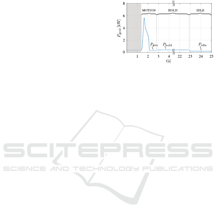
Figure 1: Typical power consumption measurement for an
industrial robot in different operating phases.
2 MODEL OF SYSTEM ENERGY
Comprehensive energy demand modelling ap-
proaches for mechatronic systems have been
presented in earlier publications (Hansen et al., 2013;
Pellicciari et al., 2013). However, the proposed
model is specifically designed for industrial robots,
which enables significant model complexity reduc-
tions without perceptible changes in accuracy. This
leads to advantages in feasibility, computation time,
and system identification effort. Assuming that the
parameters of the inverse dynamics model are known,
the presented power model uses only three additional
parameters that can be identified in a single mea-
surement. The correct simulation and comparison
of the energy consumption for different travel times
requires a model representing the consumption while
in motion as well as in standstill. In order to clarify
the different power consumption phases, a typical
power measurement for a PTP motion is shown in
Figure 1. The operational state can be divided into
three different phases:
• MOTION means that the robot is currently moving,
• HOLD describes a robot in active control with
lifted holding brakes, while
• IDLE signifies that the holding brakes have been
applied.
The causes for the power consumption in the dif-
ferent phases are explained in section 2.1, along with
the identification of the required parameters. The
modelling of the motion-dependent power consump-
tion is formulated in section 2.2. Validation measure-
ments are presented in section 2.3.
2.1 Operating Phases
The power consumption during the different operat-
ing phases can be explained by consideration of a
ICINCO 2017 - 14th International Conference on Informatics in Control, Automation and Robotics
528
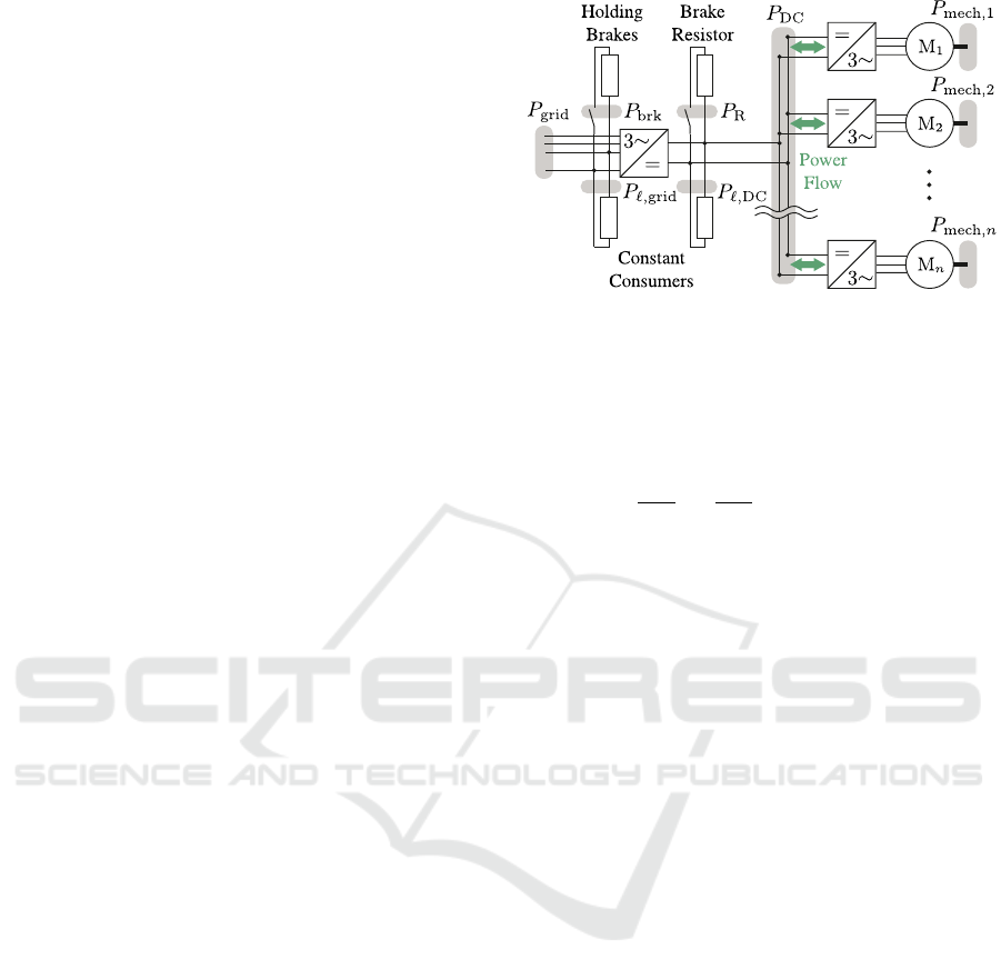
simplified electrical substitute circuit diagram (Fig-
ure 2). During the MOTION phase, the power con-
sumption depends on the robot’s mechanical power
demand P
mech,i
that is induced by the given motion.
A detailed description of the modelling approach for
this particular term can be found in section 2.2. The
sum of mechanical powers is represented by an aux-
iliary variable P
DC
that characterizes the power flow
within the DC bus. Since most state-of-the-art robot
controls are not able to recuperate, excess power P
R
is
dissipated through a brake resistor. All further DC bus
losses are summarized as a constant loss power P
`,DC
.
Constant losses on the grid side are split into two
groups: the power P
brk
is required to keep the brakes
lifted while P
`,grid
summarizes the constant losses of
all peripheral components (e. g. controller, cooling
fans, IO modules, sensors, etc.).
During the IDLE phase, all the components on a
600 V level are inactive and the holding brakes are
applied. Hence, the measurable power P
idle
equals
P
`,grid
. In the HOLD phase, the power demand is in-
duced by the constant losses on the grid side, on the
DC side, and by the brake lifting power:
P
hold
= P
`,grid
+ P
`,DC
+ P
brk
. (1)
The power consumption for the static holding is
not considered separately. It is instead included in
the constant DC losses P
`,DC
. The dependency on
the robot configuration is neglected: measurements
have shown a maximum deviation of P
hold
of ap-
prox. 10 % for the KUKA KR 16 and 5 % for the
KUKA KR 210 for the most extreme poses (see sec-
tion 2.3 for the test bed description). The influence for
the KR 210 is lower due to its counterbalancing sys-
tem. However, with regard to the robots’ peak powers
of approx. 8 kW (KR 16, see Figure 4) and 20 kW
(KR 210, see Figure 5), the deviation comes down to
less than 0.01 % in each case.
The utilization of substitute powers for various
losses is a major change in comparison to existing
approaches (Hansen et al., 2013; Pellicciari et al.,
2013). Industrial robots usually feature backlash free
gears with high friction. Hence, the mechanical losses
clearly exceed the electrical ones. Therefore, the pro-
posed simplifications only have a minor impact on
the grid power consumption (see also section 2.3).
The main advantage of this approach is the signifi-
cant reduction of required parameters which enables
the model for application on an industrial level.
2.2 Motion-dependent Power
Consumption
This section focuses on the calculation of the motion-
dependent power consumption. Assuming that a tra-
Figure 2: Electrical substitute circuit diagram for an indus-
trial robot.
jectory of an industrial robot is predefined, the calcu-
lation of the system power demand starts with deter-
mining the motor torques τ (t). In general, the model
for inverse dynamics is given by
τ (t) =diag(
1
u
G,1
,...,
1
u
G,n
)(M (q)¨q + c(q, ˙q) + g(q))
+ h(q, ˙q), (2)
where q, ˙q, ¨q are time-dependent joint angles, veloc-
ities, and accelerations given by the trajectory plan-
ning algorithm. The term u
G,i
represents the gear fac-
tor for joint i while the vector τ contains the respec-
tive motor torques τ
i
. M contains moments of inertia,
c Coriolis effects, and g gravitational effects. h sum-
marizes non-linear effects which in our regarded case
is merely friction. In (Hamon et al., 2010), a com-
monly used friction model including Coulomb fric-
tion and viscous damping (coefficients f
c,i
and f
v,i
,
respectively) is presented. It is applied for this model,
expressing friction torque τ
f,i
for joint i as
τ
f,i
(t) = h
i
(t) = f
c,i
sign(
˙
ω
i
(t)) + f
v,i
˙
ω
i
(t), (3)
where ω
i
is the angular motor velocity of motor i
which can be determined as
ω
i
(t) = u
G,i
˙q
i
(t). (4)
Most robotic manufacturers utilize a model of the
inverse dynamics within the robot control system for
implementation of feed forward control. Thus, it can
be assumed that the system friction parameters are
known. If not, they can be obtained using established
identification methods (Johnson and Lorenz, 1992).
Equations 2 and 4 are used to obtain the mechanical
power P
mech,i
(t) for each motor i:
P
mech,i
(t) = τ
i
(t) ω
i
(t). (5)
The The total DC bus power P
DC
is obtained by
summing up the mechanical power of the n individual
motors:
P
DC
(t) =
n
∑
i=1
P
mech,i
(t). (6)
Optimizing PTP Motions of Industrial Robots through Addition of Via-points
529
For state-of-the-art industrial robots, the DC bus
features a capacitor that is usually dimensioned to
smoothen the rectified voltage, not to buffer excess
energy in generator operation phases. Therefore, the
capacity is neglected. However, it can be imple-
mented according to (Hansen et al., 2012) if desired.
Further, the rectifiers in industrial robot cabinets are
usually not able to recuperate. Hence, negative values
for P
DC
need to be partly corrected. The excess power
in generator operating phases can cover the constant
losses within the DC bus, but the grid side losses will
remain. The remaining power consumption is marked
as P
gen
in Figure 1. This behaviour is considered as
follows:
P
DC
(t) + P
`,DC
≥ 0 :
P
grid
(t) = P
DC
(t) + P
`,DC
+ P
`,grid
+ P
brk
,
P
R
(t) = 0,
P
DC
(t) + P
`,DC
< 0 :
P
grid
(t) = P
gen
= P
`,grid
+ P
brk
,
P
R
(t) = −(P
DC
(t) + P
`,DC
),
where P
R
(t) is the power dissipated via the brake
resistor. The time integral of the grid power demand
over trajectory time (from t
start
to t
end
)
E
grid
=
Z
t
end
t
start
P
grid
(t) dt (7)
equals the grid energy demand of the system for a
given trajectory.
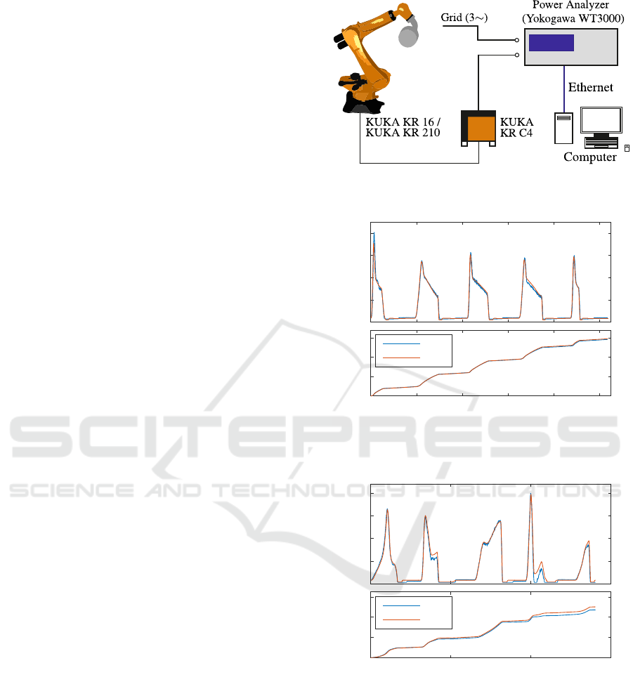
2.3 Validation
In order to demonstrate its portability, the model is ap-
plied to and parameterized for two robots of different
sizes, namely a KUKA KR 16 and a KUKA KR 210
with respective payloads of 16 kg and 210 kg. The test
setup for the validation is shown in Figure 3. The grid
power is measured using a Yokogawa WT 3000 pre-
cision power analyzer. The robots are equipped with
a test weight of 15 kg and 200 kg.
The Figures 4 and 5 show the measured as well as
the simulated power demand and the grid energy de-
mand for both robots. The validation trajectory con-
sists of five PTP motions, separated by one-second
pauses. The resulting grid energy demand for the
KR 210 is slightly overestimated by the simulation by
+5.3 %. At about 10 s, the power demand differs a lit-
tle bit more extreme than for the other motions. This
might occur due to inaccuracies in the robot control’s
inverse dynamic model for this exact movement.
For the KR 16, the simulation provided an even lower
deviation of 1.2 % for the given trajectory. Fur-
ther measurements with varying trajectories delivered
Figure 3: Test setting for validation trajectory measurement;
figures are properties of the respective manufacturers.
0
2
4
6
8
P
grid
[kW]
KUKA KR 16
0 2 4 6 8 10
t [s]
0
5
10
15
E
grid
[kJ]
meas.
sim.
Figure 4: Measured and simulated power demand for the
KUKA KR 16.
0
5
10
15
20
P
grid
[kW]
KUKA KR 210
0 5 10 15
t [s]
0
20
40
60
E
grid
[kJ]
meas.
sim.
Figure 5: Measured and simulated power demand for the
KUKA KR 210.
comparable results with an error within approx. ±
5 %. The validation results show that the model with
the proposed complexity reductions, in contrast to in-
creasingly complex models in the current develop-
ment of research, adequately depicts the real system’s
grid power and energy demand.
While different simplifications have been intro-
duced for the modelling of the electrical part of the
drive system, it is important to reach a high accuracy
ICINCO 2017 - 14th International Conference on Informatics in Control, Automation and Robotics
530
0 1 2 3 4 5
t [s]
-2
0
2
4
6
P
mech;1
[kW]
#
1
= 20
/
C
#
1
= 70
/
C
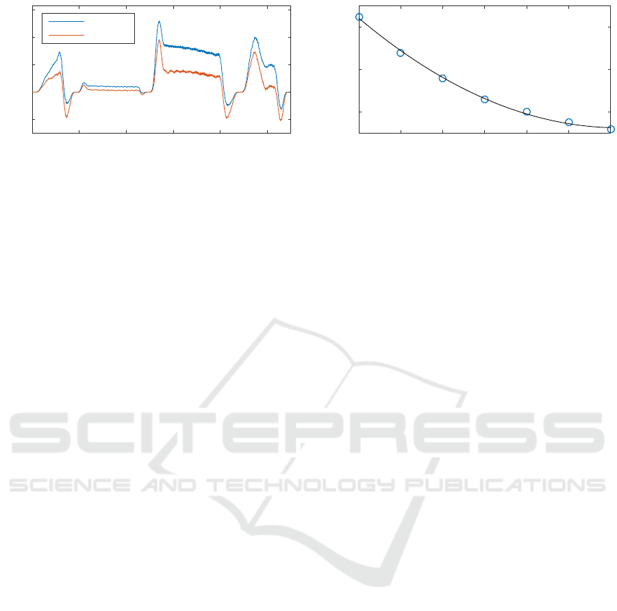
Figure 6: Mechanical power comparison for axis i = 1 at
different motor temperatures based on measured (traced)
values for τ
1
and ω
1
.
for the calucation of the mechanical power. Although
there is a strong dependency between robot tempera-
ture and its power demand, previous works often ne-
glect this. While (Brossog et al., 2015),(Meike et al.,
2014) consider the robot temperature, only the tem-
perature dependencies of motor resistors are taken
into account.
Figure 6 demonstrates the impact of the robot (i. e.
motor) temperature on the mechanical power. The
values are based on the traced values at a KR 210 us-
ing its internal sensors. While the motor temperature
ϑ
i
does not equal the gear temperature, it sufficiently
displays the robot’s thermal state. The measured grid
energy consumption for the same motion at different
temperatures is shown in Figure 7. It becomes ob-
vious that a consideration of the temperature within
the model is inevitable. Therefore, the model should
either utilize temperature-dependent friction parame-
ters or they need to be identified for a task-specific
thermal state. For this paper, the friction parameters
were identified for motor temperatures of 60
◦
C. Un-
less stated otherwise, all presented measurements and
results refer to this operating point.
3 OPTIMIZATION APPROACH
The following section describes state-of-the-art tra-
jectory planning implemented in several standard in-
dustrial robot control systems. Following, the pro-
posed approach to modify trajectories towards less
energy consumption is introduced. Additionally, op-
timization of travel time is considered. Furthermore,
the optimization method including its cost functions
and boundaries are presented.
3.1 Standard Trajectory Planning
A common solution for PTP trajectory planning is
based on trapezoidal acceleration profiles with syn-
20 30 40 50 60 70 80
#
1
[
/
C]
1
1.2
1.4
E
grid
=E
grid;60
Figure 7: Dependency of grid energy demand E
grid
on tem-
perature normalized to the grid energy demand E
grid,60
at
60
◦
C motor temperature.
chronously moving axes (Biagiotti and Melchiorri,
2008). This results in continuous joint angle, velocity,
and acceleration functions, but in a non-continuous
jerk function. However, the actual acceleration func-
tions of modern robot controls differ from strict trape-
zoidal profiles to further improve travel time. Accel-
eration is constrained by the maximum torque lim-
its of the axes (Costantinescu and Croft, 2000). This
leads to at least one axis reaching its torque limit,
as shown in the results section. All axes move syn-
chronously.
3.2 Trajectory Modification by adding
Via-Points
By adding via-points we are able to modify a given
trajectory towards optimized energy consumption
and/or travel time. The advantage of this method,
in contrast to previous works using spline interpola-
tion such as (Meike and Ribickis, 2011),(You et al.,
2011),(Hansen et al., 2012), is the simple implemen-
tation to commercial robot controls. The method ex-
clusively utilizes standard control commands. Ini-
tially, this seems paradoxical since adding via-points
seem like a detour on the way from starting to final
configuration. However, if the via-points are placed
in an certain position, a configuration with reduced
moments of inertia M(q) can result. According to
(2), a reduction of M (q) can be exploited to
• increase joint acceleration at equal joint torque or
• decrease joint torque at equal joint acceleration.
Possible benefits are pointed out in the following
two scenarios: Assuming the user wants to lower en-
ergy consumption for a given PTP motion without
changing the travel time, lower joint torques can de-
crease the total energy demand, whereas maintaining
equal acceleration keeps the travel time constant.
Alternatively, the user wants to lower travel time
for a given PTP motion. This could be accomplished
Optimizing PTP Motions of Industrial Robots through Addition of Via-points
531

by increasing joint acceleration, which is limited by
maximum joint torque, as described in section 3.1.
Thanks to the reduced moment of inertia in via-point
configuration compared to the initial trajectory, accel-
eration can be increased without exceeding the torque
limits.
The addition of via-points can also desynchro-
nize the axes’ movement. Non-synchronously mov-
ing axes allow the usage of recuperated energy from
deceleration phases through DC-bus linkage, which
leads to a reduction of dissipated energy and, there-
fore, to a higher overall energy efficiency. Figure 2
shows the corresponding energy flows.
Any number of via-points can be added to the ini-
tial trajectory. However, in order to assure a sim-
ple understanding we present our methods and results
based on the addition of one via point. Note that more
via-points increase the computational expense due to
the increased dimension of the optimization parame-
ter vector.
Furthermore, apart from the optimization of en-
ergy consumption, other targets can be considered by
replacing the cost function. As the optimization of
travel time is often addressed in previous works, it is
additionally considered in this paper.
3.3 Optimization Method
The initial trajectory with synchronously moving axes
as described in section 3.1 is programmed in robot
control as shown in Figure 8. It represents a PTP
motion from starting joint angle configuration q
s
to
end configuration q
e
. Velocity and acceleration are
set to maximum (100 %) which are the default values
in most common robot control systems.
The optimization target is set by defining the cost
function. Basically, any type of cost function can be
formulated. Following, we focus on reduction of en-
ergy consumption and additionally travel time.
3.3.1 Optimization of Energy Consumption
The optimization parameter vector
p
e
= (p
1
, p
2
,..., p
n
|
{z }
p
e,joint config.
,v,a)
T
(8)
contains all n joint angles of the via-point added to the
initial trajectory between start and end configuration,
velocity v, and acceleration a. Velocity and accelera-
tion are expressed in percentage of the respective set
maximums.
The initial as well as the temporary trajectories of
iteration steps, are generated using original trajectory
planning of the robot control system. This is realized
1 for i=1 to 6
2 $acc axis[i]=100 initial accel. and velocity
3 $vel axis[i]=100 settings in %
4 endfor
5
6
7
8 Points for PTP motion in joint space
9 PTP {A1 q
s,1
, A2 q
s,2
, A3 q
s,3
, A4 q
s,4
, A5 q
s,5
,
A6 q
s,6
}
10
11 PTP {A1 q
e,1
, A2 q
e,2
, A3 q
e,3
, A4 q
e,4
, A5 q
e,5
,
A6 q
e,6
}
Figure 8: Trajectory Source Code in Kuka Robot Language.
by including hardware in the loop of optimization.
This method of trajectory generation automatically
satisfies all constraints like maximum motor torques,
maximum gear torques, maximum joint velocities set
by the robot manufacturer. It also allows to simply
implement the optimized trajectory in the robot con-
trol by using standard commands. In contrast, if the
trajectory is interpolated e.g. using B-splines, this
becomes more problematic. The resulting joint an-
gles q(t), velocities ˙q(t), and accelerations ¨q(t) are
then used to calculate the energy consumption of the
motion as described in section 2.2. The optimization
problem is formulated as a minimization of total en-
ergy demand
p
∗
e
= argmin
p
e
E
grid
(q
s
,p
e
,q
e
)
, (9)
where p
∗
e
is the optimal parameter vector. All param-
eters’ upper and lower bounds are
q
i,min
≤ p
i
≤ q
i,max
∀ i = 1... n, (10)
0% ≤ v ≤ 100 %, (11)
0% ≤ a ≤ 100 %, (12)
where limits to p
i
originate from kinematic con-
straints, preventing the robot from colliding with ob-
stacles or itself. Additionally, a non-linear constraint
t
temp
≤ t
thr
(13)
is implemented to ensure that the travel time of the
temporary optimized trajectory t
temp
in each iteration
does not impair the threshold travel time t
thr
. Thresh-
old travel time commonly is the travel time of the ini-
tial trajectory t
init
.
3.3.2 Optimization of Travel Time
In contrast, if the target is to optimize the travel time,
the optimization parameter vector slightly changes to
p
t
=
p
1
, p
2
,..., p
n
T
. (14)
ICINCO 2017 - 14th International Conference on Informatics in Control, Automation and Robotics
532

1 for i=1 to 6
2 $acc axis[i]=a
∗
opt. acceleration and velocity
3 $vel
axis[i]=v
∗
settings in %
4 endfor
5
6 $apo.
cptp
=100 via-point approx. set to max.
only affects points between
start and end configuration
7
8 Points for PTP motion in joint space
9 PTP {A1 q
s,1
, A2 q
s,2
, A3 q
s,3
, A4 q
s,4
, A5 q
s,5
,
A6 q
s,6
}
10 PTP {A1 p
∗
1
, A2 p
∗
2
, A3 p
∗
3
, A4 p
∗
4
, A5 p
∗
5
,
A6 p
∗
6
}
c ptp
11 PTP {A1 q
e,1
, A2 q
e,2
, A3 q
e,3
, A4 q
e,4
, A5 q
e,5
,
A6 q
e,6
}
Figure 9: Optimized Trajectory Source Code.
In this case, the optimization process has no influ-
ence on velocity and acceleration settings, as minimal
travel time arises from both variables set to their max-
imum of
v = v
max
= 100%, (15)
a = a
max
= 100%. (16)
Again, trajectories are generated utilizing the orig-
inal trajectory planning from the robot control. This
includes calculation of travel time t
trav
. The resulting
cost function is
p
∗
t
= argmin
p
t
(t
trav
(q
s
,p
t
,q
e
)) (17)
and does not include the model of system energy in
section 2. Parameter bounds are the same as defined
in (10), respectively.
Additional non-linear constraints can be consid-
ered to further tune the trajectory according to re-
quired characteristics. For instance, in order to re-
strict the deviation of the optimized trajectory from
the initial, a constraint to ensure the optimized tra-
jectory stays in bounds of a tube with a defined radius
around the initial trajectory can be used (Hussong and
Heimann, 2007).
Analogically, any kind of restriction can be con-
sidered, however, additional non-linear constraints
can lead to less flexibility for the optimization which
leads to less advance in performance. Improvement
possibilities depend on the initial trajectory and the
workspace circumstances.
3.3.3 Optimization Procedure
The non-linear optimization problem is solved using
an active-set algorithm. The starting point for opti-
mization is set in the middle (in joint space) between
start and end configuration
p
start
e,joint config.
= p
start
t
=
q
s
+ q
e
2
. (18)
The resulting optimal parameter vector is then used
to optimize the robot control program. In case of
the addition of multiple via-points, starting points are
equidistantly distributed.
The whole optimization process runs automati-
cally. A robot control program on a KUKA KR C4
is read and relevant information is extracted. Then,
the actual optimization process is performed. After-
wards, a robot control program, including the added
resulting via-points, is generated. Exemplary, a re-
sulting optimized code for a single added via-point is
shown in Figure 9.
4 RESULTS
This section presents optimization results for differ-
ent PTP trajectories on the KUKA KR 210 industrial
robot, shown in Figure 10. The model of system en-
ergy in section 2 and the optimization method in sec-
tion 3 are applied. All trajectories analyzed include an
additional test load of 200 kg mounted at the robot’s
end-effector flange.
Furthermore, initial trajectories move with max-
imum velocity and acceleration, as it is a standard
in industrial application to achieve minimum travel
times.
Like many other high-payload robots, the KR 210
has a counterbalancing system between axis 1 and
2. This lowers high torque demands for axis 2 in
Table 1: Start and End Configurations (in Degrees) of the
PTP Trajectories with Energy and Time Optimized Via-
Points.
T1
q
T
s
= [ 0.0 -5.0 0.0 0.0 0.0 0.0 ]
q
T
via,e
= [ -2.2 -69.8 6.9 4.0 -67.9 1.4 ]
q
T
via,t
= [ -0.3 -69.9 -42.7 0.4 -105.8 0.0 ]
q
T
e
= [ 0.0 -140.0 0.0 0.0 0.0 0.0 ]
T2
q
T
s
= [-150.0 -5.0 -90.0 -45.0 -50.0 -45.0 ]
q
T
via,e
= [ -18.6 -51.4 -15.2 74.1 65.8 25.6 ]
q
T
via,t
= [ -9.3 -39.9 -38.7 61.1 96.0 22.1 ]
q
T
e
= [-150.0 -90.0 90.0 180.0 125.0 120.0 ]
T3
q
T
s
= [ -55.0 -5.0 10.0 100.0 10.0 -40.0 ]
q
T
via,e
= [ -28.0 -39.0 -23.6 -21.1 125.0 54.2 ]
q
T
via,t
= [ -22.3 -53.1 -26.9 -40.1 55.0 5.3 ]
q
T
e
= [ 15.0 -105.0 -60.0 -180.0 100.0 50.0 ]
T4
q
T
s
= [-165.0 -115.0 -110.0 -316.0 -114.0 -316.0 ]
q
T
via,e
= [ 16.5 -55.1 27.2 -4.7 47.1 -10.6 ]
q
T
via,t
= [ 17.2 -51.2 26.6 -13.5 6.4 -14.3 ]
q
T
e
= [ 166.0 -9.0 111.0 319.0 115.0 319.0 ]
Optimizing PTP Motions of Industrial Robots through Addition of Via-points
533

stretched configurations. The influence of the coun-
terbalancing system on the robot is included in the
dynamic model (Hansen et al., 2012).
Table 1 shows exemplary chosen PTP trajecto-
ries including their starting and ending configurations.
The trajectories cover different motion characteris-
tics, such as horizontal and vertical motion, a combi-
nation of both and an all axis motion from minimum
to maximum joint angle limit.
Additionally, the axis configurations of optimized
via-points q
∗
e,via
and q
∗
t,via
for energy-optimized PTP
motions are presented. Associated velocity and ac-
celeration values are v
T1
= 74.7 %, v
T2
= 80 %, v
T3
=
72%, and v
T4
= 80 %, whereas acceleration stays at
almost 100 % for all four trajectories.
Table 2: Results for Energy and Time Optimized Trajec-
tories. The Colors, Associated to Figure 10, Highlight the
Results.
Travel
Time [s]
Energy
Cons. [J]
Time-Opt.
Slowed [J]
T1
init
2.96 9733
T1
opti,e
2.96 8060 (-17.2 %)
T1
opti,t
2.57 (-13.3 %) 9476 (- 2.6 %) 8195 (-15.8 %)
T2
init
3.50 15005
T2
opti,e
3.50 12992 (-13.4 %)
T2
opti,t
3.09 (-11.7 %) 15751 (+ 5.0 %) 13535 (- 9.8 %)
T3
init
3.01 11769
T3
opti,e
3.01 9678 (-17.3 %)
T3
opti,t
2.85 (- 5.33 %) 13841 (+ 17.7 %)11345 (- 3.6 %)
T4
init
4.84 30268
T4
opti,e
4.84 26692 (-11.8 %)
T4
opti,t
4.44 (- 8.3 %) 30251 (- 0.1 %) 27422 (- 9.4 %)
The resulting energy savings are summarized in
Table 2. For the exemplary chosen trajectories, we
achieve energy savings up to 17.3 %.
In order to clarify the effects leading to the im-
provement, T1 is analyzed in detail. Figure 11 shows
initial and energy-optimized joint motor torques of
T1. As mentioned in 3.1, torque limited trajectory
generation leads to at least one axis reaching its max-
imum torque limit. Even though only axis 2 is sup-
posed to move, the other horizontal axes have to com-
pensate torques due to moments of inertia, Coriolis
and gravitational effects. For T1, axes 3 and 5 even
reach their torque limits. The added via-point of the
energy-optimized trajectory allows the axes torques to
be lowered more quickly. Axes 2 and 5 cross the zero
torque level approximately 0.4 s earlier than the ini-
tial trajectory. Overall reduced torques lead to energy
savings of 17.2 %. Retardations are prevented due to
the applied boundaries.
Alternatively, the cost function can be exchanged
to minimize the travel time. Optimization of travel
time is performed as an example for other optimiza-
tion targets. Time savings up to approximately 13 %
are accomplished.
Initial and time-optimized joint velocities of T1 in
Figure 11 allow for a closer look at the time optimiza-
tion. Standard trajectory planning for a difference be-
tween start and end configuration in only one axis, in
this case axis 2, results in a single movement of that
axis. In contrast, the optimized trajectory shows an
additional movement of the previously passive axes,
especially the parallel ones. The additional motions
lead to an optimized configuration regarding moments
of inertia, Coriolis and gravitational effects. Regard-
ing axis 2, this allows for a motion with increased ve-
locity after reaching its peak at about 1.6 s, leading to
time savings of 13.3 % and simultaneous energy sav-
ings of 2.6 % as a side effect.
The time savings can then be used to reduce ac-
celeration and/or velocity settings, leading to reduced
energy consumption. Hence, resulting energy savings
are included in Table 2. The energy savings of the
time-optimal slowed down trajectory come close to
the energy-optimized results, but do not reach those.
However, for optimization of travel time no model of
system energy is required.
5 CONCLUSION AND FUTURE
WORKS
5.1 Conclusion
A new approach to automatically improve PTP mo-
tions of robotic systems using standard robot control
has been presented. The proposed methods were suc-
cessfully implemented on the KUKA KR 210. The re-
sulting optimized source code differs from the initial
one only by the added via-points which can be added
using standard commands of common robot control
systems.
Exemplary, in this paper the addition of one via-
point is considered. In case of multiple via-points, the
procedure is same. The initial multiple via-points are
distributed equidistantly between start and end con-
figuration, as described in section 3.3.3, and then all
of them are optimized at the same time towards min-
imizing the respective cost function. Note that ad-
dition of multiple via-points increases the dimension
of the parameter vector by six per additional via-point
for a robot with n = 6 degrees of freedom which raises
computational expenses. However, the optimized tra-
ICINCO 2017 - 14th International Conference on Informatics in Control, Automation and Robotics
534
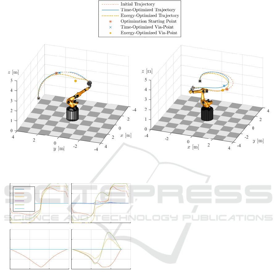
(a) Trajectory T1 (b) Trajectory T2
Figure 10: Exemplary Considered Trajectories T1 and T2.
-1
-0.5
0
0.5
1
= ==
max
T1
init
Joint Torques
Axis 1
Axis 2
Axis 3
Axis 4
Axis 5
Axis 6
T1
opti;e
Joint Torques
0 1 2 3
t [s]
-1
-0.5
0
0.5
1
v=v
max
T1
init
Joint Velocities
0 1 2 3
t [s]
T1
opti;t
Joint Velocities
Figure 11: Comparison of Initial to Energy-Optimized Joint
Motor Torques and Initial to Time-Optimized Joint Veloci-
ties of T1.
jectory could be specified more exactly which may
lead to further optimization potential.
The via-point’s configuration in joint space is cal-
culated by formulating an optimization problem. Sev-
eral optimization targets can be implemented by ex-
changing the cost function. In this paper we focus on
reducing energy consumption and additionally con-
sider optimization of travel time. Collision avoidance
can be implemented by setting non-linear constraints.
In comparison to existing approaches, our model
of system energy is more simple and requires less in-
formation of the system. However, it is suitable to
depict the energy demand of serial cinematic indus-
trial robots and to be implemented for optimization
procedure.
Based on the introduced model of system energy,
the optimization problem to reduce energy consump-
tion has been formulated. The experimental results
have shown energy savings up to 17.3 %.
In contrast, targeting to the optimization of travel
time, a different cost function has been formulated.
The implementation of this target has resulted in
time savings up to 13.3 %. These savings can also be
used, to reduce energy consumption by decreasing
acceleration and velocity settings on robot control.
Hence, energy savings up to 15.8 % are achieved.
Future works may focus on the addition of multi-
ple via-points to the initial trajectory and on the eval-
uation of the results for a high number of different ini-
tial trajectories. Furthermore, the methods presented
in this paper could be tested for different types of in-
dustrial robots.
5.2 Reduced Complexity Optimization
Method
Reviewing the resulting trajectories of the presented
approach lead to another method. Future works may
focus on the direct minimization of moment of iner-
tia. The complete model of system energy as well
Optimizing PTP Motions of Industrial Robots through Addition of Via-points
535
as the inverse dynamics are highly complex and re-
quire a lot of system information. The advantages of
reduced moments of inertia are explained in section
3.2. Following, an approach to optimize robot trajec-
tories focusing on direct minimization of moment of
inertia is proposed. In this case, the Cartesian inertia
matrix M needs to be calculated.
The cost function for this approach is
p
∗
in
= argmin
p
in
M
(ax ax)
(p
in
)
, (19)
where ax is the axis for which the moment of
inertia is to be minimized, and parameter vector p
in
equals p
t
. The chosen axis depends on the initial
trajectory. Initial and optimized robot control codes
are programmed in the same manner as shown in
section 3.3.
This approach comes along with some challenges.
The cost function does not include any information
about the resulting travel time or energy consump-
tion. Therefore, an explicit target for the optimization
can not be set.
Furthermore, reducing the moment of inertia is
not suitable for all kinds of trajectories. Those with a
significant downwards movement of the end-effector
profit from gravitational effects. This profit increases
with greater moment of inertia, as the mass of
robot links induce a joint torque in the direction of
movement and, therefore, lower the share of overall
joint torques provided by the motors.
Finally, the minimum could be a long distance away
from initial trajectory, resulting in a great detour and
no improvement in performance. However, non-
linear constraints can prevent this problem. In this
paper, the exemplary single via-point is kept inside a
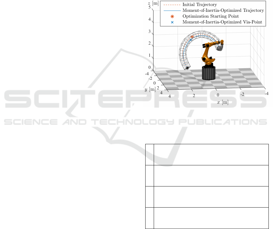
tube around the initial trajectory, as shown in Figure
12. This constraint is implemented by calculating the
via-point’s distances in workspace to all points of the
initial trajectory. The minimum of these distances is
the via-point’s distance to the trajectory and it must
not exceed the tube radius. Besides, it allows not
only a radial shift of the via-point, but in any three
dimensional direction.
Experimental Results
The aforementioned approach is applied to the
trajectories previously considered in this paper. To
avoid the problem of excessive detours, an additional
non-linear constraint is implemented. This constraint
keeps the optimized via-point inside a tube with
a radius of r = 0.3 m around the initial trajectory.
However, this only represents a possible first solution
for the problems pointed out before and the settings
of that constraint also depend robot and trajectory
characteristics. The optimized via-points for each
trajectory are presented in Table 3, associated energy
and time savings are listed in Table 4. Minimizing
the moment of inertia in via-point configuration has
shown time savings up to 9.6 % and energy savings
up to 6.3 %. Initial and optimized trajectory T3 in
workspace are shown in Figure 12. Although this
approach cannot set a specific target, it requires less
information of the system and significantly lowers
computational time of the optimization.
Figure 12: Initial and Moment of Inertia Optimized Trajec-
tory T3.
Table 3: Start and End Configurations of the PTP Trajecto-
ries with their Moment of Inertia Optimized Via-Points.
T1
q
T
s
= [ 0.0 -5.0 0.0 0.0 0.0 0.0 ]
q
T
via,in
= [ -0.0 -63.1 -50.0 28.6 -50.0 -6.8 ]
q
T
s
= [ 0.0 -140.0 0.0 0.0 0.0 0.0 ]
T2
q
T
s
= [-150.0 -5.0 -90.0 -45.0 -50.0 -45.0 ]
q
T
via,in
= [ 0.1 -49.1 -0.90 1.8 151.7 170.0 ]
q
T
e
= [-150.0 -90.0 90.0 180.0 125.0 120.0 ]
T3
q
T
s
= [-55.0 -5.0 10.0 100.0 10.0 -40.0 ]
q
T
via,in
= [-20.0 -55.0 -25.0 -6.6 150.0 100.0 ]
q
T
e
= [ 15.0 -105.0 -60.0 -180.0 100.0 50.0 ]
T4
q
T
s
= [-165.0 -115.0 -110.0 -316.0 -114.0 -316.0]
q
T
via,in
= [ 0.5 -62.0 0.5 2.0 -147.4 -0.1 ]
q
T
e
= [166.0 -9.0 111.0 319.0 115.0 319.0 ]
The results show that the approach of reducing
moment of inertia is more suitable to optimize tra-
jectories’ travel time at this stage. To obtain optimal
configuration concerning moment of inertia, given the
previously mentioned constraints, major additional
axes motion is necessary. This may lead to higher
energy demand, e. g. for trajectories T1 and T2.
However, T3 and T4 show that further development
ICINCO 2017 - 14th International Conference on Informatics in Control, Automation and Robotics
536

may enable to optimize energy consumption and
travel time simultaneously. Furthermore, the reduced
complexity cost function favors the possibility of
online application. Suitable constraints to develop
this approach need to be addressed in future works.
Table 4: Results for Moment of Inertia Optimized Exem-
plary Trajectories.
Travel
Time [s]
Energy
Consumption [J]
T1
init
2.96 9733
T1
opti,in
2.78 (- 6.1 %) 10394 (+ 6.8 %)
T2
init
3.50 15005
T2
opti,in
3.20 (- 8.6 %) 16193 (+ 7.9 %)
T3
init
3.01 11769
T3
opti,in
2.72 (- 9.6 %) 11021 (- 6.4 %)
T4
init
4.84 30268
T4
opti,in
4.57 (- 5.6 %) 28492 (- 5.9 %)
ACKNOWLEDGEMENTS
The authors would like to thank the KUKA Roboter
GmbH for granting us access to their laboratories to
perform power measurements on a KUKA KR 210.
REFERENCES
(2016). World record: 248.000 industrial robots revolution-
ising the global economy. IFR press release.
Biagiotti, L. and Melchiorri, C. (2008). Trajectory Planning
for Automatic Machines and Robots. Springer Science
& Business Media.
Bobrow, J. E. (1988). Optimal Robot Plant Planning Us-
ing the Minimum-Time Criterion. IEEE Journal on
Robotics and Automation, 4(4):443–450.
Brossog, M., Bornschlegl, M., Franke, J., et al. (2015). Re-
ducing the Energy Consumption of Industrial Robots
in Manufacturing Systems. The International Jour-
nal of Advanced Manufacturing Technology, 78(5-
8):1315–1328.
Costantinescu, D. and Croft, E. (2000). Smooth and time-
optimal trajectory planning for industrial manipula-
tors along specified paths. Journal of Robotic Systems,
17(5):233–249.
Gattringer, H., Riepl, R., and Neubauer, M. (2013). Op-
timizing Industrial Robots for Accurate High-Speed
Applications. Journal of Industrial Engineering,
2013.
Geering, H. P., Guzzella, L., Hepner, S. A., and Onder, C. H.
(1985). Time-Optimal Motions of Robots in Assem-
bly Tasks. In Proc. of the IEEE Conf. on Decision and
Control, pages 982–989.
Gleeson, D., Bj
¨
orkenstam, S., Bohlin, R., Carlson, J. S., and
Lennartson, B. (2015). Optimizing Robot Trajectories
for Automatic Robot Code Generation. In Proc. of the
IEEE Int. Conf. on Automation Science and Engineer-
ing, pages 495–500. IEEE.
Gleeson, D., Bj
¨
orkenstam, S., Bohlin, R., Carlson, J. S., and
Lennartson, B. (2016). Towards Energy Optimiza-
tion Using Trajectory Smoothing and Automatic Code
Generation for Robotic Assembly. Procedia CIRP,
44:341–346.
Hamon, P., Gautier, M., and Garrec, P. (2010). Dy-
namic Identification of Robots With a Dry Friction
Model Depending on Load and Velocity. In Proc. of
the IEEE/RSJ International Conference on Intelligent
Robots and Systems, pages 6187–6193.
Hansen, C., Eggers, K., Kotlarski, J., and Ortmaier, T.
(2015). Concurrent Energy Efficiency Optimization
of Multi-Axis Positioning Tasks. In Proc. of the IEEE
Int. Conf. on Industrial Electronics and Applications,
pages 518–525.
Hansen, C., Kotlarski, J., and Ortmaier, T. (2013). Path
Planning Approach for the Amplification of Electri-
cal Energy Exchange in Multi Axis Robotic Systems.
In Proc. of the IEEE Int. Conf. on Mechatronics and
Automation, pages 44–50.
Hansen, C.,
¨
Oltjen, J., Meike, D., and Ortmaier, T. (2012).
Enhanced Approach for Energy-Efficient Trajectory
Generation of Industrial Robots. In Proc. of the IEEE
Int. Conf. on Automation Science and Engineering,
pages 1–7.
Hussong, A. and Heimann, B. (2007). Restricted Minimum-
Effort Motion Planning for serial Manipulators. In
Proceedings of the 12th IFToMM World Congress.
Johnson, C. T. and Lorenz, R. D. (1992). Experimental
identification of friction and its compensation in pre-
cise, position controlled mechanisms. IEEE Transac-
tions on Industry Applications, 28(6):1392–1398.
Meike, D., Pellicciari, M., and Berselli, G. (2014). Energy
Efficient Use of Multirobot Production Lines in the
Automotive Industry: Detailed System Modeling and
Optimization. IEEE Transactions on Automation Sci-
ence and Engineering, 11(3):798–809.
Meike, D. and Ribickis, L. (2011). Industrial Robot Path
Optimization Approach with Asynchronous Fly-By in
Joint Space. In Proc. of the IEEE International Sym-
posium on Industrial Electronics, pages 911–915.
Mohammed, A., Schmidt, B., Wang, L., and Gao, L.
(2014). Minimizing Energy Consumption for Robot
Arm Movement. Procedia CIRP, 25:400–405.
Paes, K., Dewulf, W., Vander Elst, K., Kellens, K., and
Slaets, P. (2014). Energy Efficient Trajectories for an
Industrial ABB Robot. Procedia CIRP, 15:105–110.
Pellicciari, M., Berselli, G., Leali, F., and Vergnano, A.
(2013). A method for reducing the energy consump-
tion of pick-and-place industrial robots. Mechatron-
ics, 23(3):326–334.
Riazi, S., Bengtsson, K., Wigstr
¨
om, O., Vidarsson, E., and
Lennartson, B. (2015). Energy Optimization of Multi-
Robot Systems. In Proc. of the IEEE Int. Conf. on Au-
tomation Science and Engineering, pages 1345–1350.
Optimizing PTP Motions of Industrial Robots through Addition of Via-points
537

Vergnano, A., Thorstensson, C., Lennartson, B., Falk-
man, P., Pellicciari, M., Leali, F., and Biller, S.
(2012). Modeling and Optimization of Energy Con-
sumption in Cooperative Multi-Robot Systems. IEEE
Transactions on Automation Science and Engineer-
ing, 9(2):423–428.
Wigstrom, O., Lennartson, B., Vergnano, A., and Brei-
tholtz, C. (2013). High-Level Scheduling of Energy
Optimal Trajectories. IEEE Transactions on Automa-
tion Science and Engineering, 10(1):57–64.
You, W., Kong, M., and Sun, L. (2011). Optimal Motion
Generation for Heavy Duty Industrial RobotsControl
Scheme and Algorithm. In Proc. of the IEEE Int. Conf.
on Mechatronics, pages 528–533.
ICINCO 2017 - 14th International Conference on Informatics in Control, Automation and Robotics
538
