Aircraft Attitude Determination Algorithms Employing Gravity Vector

Estimations and Velocity Measurements

ul de Celis and Luis Cadarso

European Institute for Aviation Training and Accreditation (EIATA), Rey Juan Carlos University,

28943 Fuenlabrada, Madrid, Spain

Keywords:

IMU, GNSS, Attitude Determination, Sensor Model, Projectile, Terminal Guidance.

Abstract:

Precision on Navigation, Guidance and Control of aircraft is dependent on the precision of the measurement

system both for position and attitude. It is well known in aerospace engineering that the rotation of an aircraft

or space vehicle can be determined measuring two vectors in two different reference systems. Velocity vector

in an aerospace vehicle can be determined in an inertial reference frame directly from a GNSS-based sensor.

Also this velocity vector can be determined by integrating the acceleration measurements in an aircraft body

ﬁxed reference frame. By estimating gravity vector in an inertial reference frame, which currently is perfectly

tabulated, and in a body reference frame, and combining these measurements with the velocity vector, rotation

of the body can be determined. Application of these concepts is especially interesting in order to substitute

high-precision attitude determination devices, which are usually expensive as they are forced to bear high

solicitations as for instance G forces.

1 INTRODUCTION

Obtaining precise attitude information is essential for

navigation and control. The effectiveness of naviga-

tion and control is determined by the degree of preci-

sion of the navigation and control systems, including

inertial measurement units (Ma et al., 2011). There is

an extensive body of literature regarding attitude es-

timation using various sensor inputs (Crassidis et al.,

2007).

Traditionally, in order to obtain accurate values

for determining attitude, expensive and/or weighty

units, such as as laser or ﬁber optic gyroscopes and

accelerometers, or their MEMS equivalents, must

be employed. High-performance electro-static gy-

roscopes require expensive vacuum-packaging, to

maintain the high-Q of the MEMS (Ismail et al.,

2015). Moreover, when high-demanding maneuvers

are performed this equipment may become extremely

expensive.

It is well-known that the attitude of an aero-

vehicle can be determined by integrating the angular

rates (pitch, roll, and yaw rates) of the vehicle. Never-

theless, accuracy requirements usually cannot be sat-

isﬁed by using the inexpensive sensors (Ma et al.,

2011). This problem becomes even more important

when the vehicle cannot be reused: low-cost attitude

determination systems are of key importance for these

applications. For example, (Gebre-Egziabher et al.,

2000) describe an attitude determination system that

is based on two vector measurements of non-zero,

non-co-linear vectors. Using the Earth’s magnetic

ﬁeld and gravity as the two measured quantities, a

low-cost attitude determination system is proposed.

(Gebre-Egziabher et al., 1998) develop an inexpen-

sive Attitude Heading Reference System for general

aviation applications by fusing low cost automotive

grade inertial sensors with GPS. The inertial sen-

sor suit consists of three orthogonally mounted solid

state rate gyros. (Eure et al., 2013) describe an atti-

tude estimation algorithm derived by post-processing

data from a small low cost Inertial Navigation System

recorded during the ﬂight of a sub-scale commercial

off the shelf UAV. Estimates of the UAV attitude are

based on MEMS gyro, magnetometer, accelerometer,

and pitot tube inputs. (Henkel and Iafrancesco, 2014)

state that low-cost GNSS receivers and antennas can

provide a precise attitude and drift-free position in-

formation, but accuracy is not continuous. Inertial

sensors are robust to GNSS signal interruption and

very precise over short time frames, which enables

a reliable cycle slip correction, but low-cost inertial

sensors suffer from a substantial drift. The authors

propose a tightly coupled position and attitude deter-

mination method for two low-cost GNSS receivers, a

gyroscope and an accelerometer and obtain a heading

Celis, R. and Cadarso, L.

Aircraft Attitude Determination Algorithms Employing Gravity Vector Estimations and Velocity Measurements.

DOI: 10.5220/0006393203770385

In Proceedings of the 14th International Conference on Informatics in Control, Automation and Robotics (ICINCO 2017) - Volume 1, pages 377-385

ISBN: 978-989-758-263-9

377

with an accuracy of 0.25

◦

/baseline length [m] and an

absolute position with an accuracy of 1 m. Similar de-

velopments may be found within space vehicles, for

example in (Springmann and Cutler, 2014).

However, as stated in (Yun et al., 2008), many of

the presented methods such as the ones employing lo-

cal magnetic ﬁeld vectors, are only valid for estimat-

ing the orientation of a static or slow-moving rigid

body. In the research described in this paper, two

measured quantities are used to obtain attitude infor-

mation for high dynamic vehicles: speed and grav-

ity vectors. They are obtained in two different refer-

ence frames using a GNSS sensor and a strap-down

accelerometer.

1.1 Contributions

The main contribution of this paper is the develop-

ment of a novel algorithm which aims at avoiding

the use of gyroscopes, and its implicit high costs if

high precision is required (Ismail et al., 2015), in

a long term and to require lower performance gy-

roscopes for attitude determination in the immediate

term. This is pretended to decrease costs in attitude

sensors and even to improve attitude determination by

applying ﬁltering techniques, especially for artillery

device purposes, where high solicitation force condi-

tions increase the price of precise attitude determina-

tion devices such as gyroscopes.

Nonlinear simulations based on ballistic rocket

launches are performed to determine real attitude and

compare it to the estimated attitude obtained from the

algorithms. The applicability of the proposed solu-

tion for aircraft ﬂight navigation, guidance and con-

trol, and for ballistic rocket terminal guidance, where

attack and side-slip aerodynamic angles are relatively

small, is also demonstrated.

This paper is organized as follows. Section II de-

scribes the problem in detail. Section III is devoted to

ﬂight dynamics and sensor models. Section IV shows

simulations results. Finally, in Section V some con-

clusions and further work are drawn.

2 PROBLEM DESCRIPTION

Attitude determination is a fundamental ﬁeld in

aerospace engineering, as maneuvers in order to

change vehicle trajectories are governed by aerody-

namic forces, which depend directly on ship orienta-

tion angles. Furthermore, attitude in artillery rockets

terminal phase is vital as it determines factors such

as penetrability of payload or countermeasures avoid-

ability. Therefore, developing algorithms to improve

attitude determination is a cornerstone in guidance,

navigation and control research.

One of the techniques to determine attitude is to

calculate it from the director cosine matrix (DCM)

which completely determines the rotation of a body.

Two reference frames are deﬁned, one ﬁxed to the

body and another one as a reference. In order to ob-

tain the DCM, a geometrical plane deﬁned in both

reference triads must be obtained. Every geometrical

plane is deﬁned by two vectors. Therefore, knowing

the same two vectors expressed in the two reference

frames, the DCM can be calculated.

2.1 Triad Deﬁnition

Two axes systems are deﬁned in order to express

forces and moments: North-East-Down (NED) axes

and Body (B) axes. NED axes are deﬁned by sub in-

dex NED. x

NED

pointing north, z

NED

perpendicular to

NED

and pointing nadir, and y

NED

forming a clock-

wise trihedron. Body axes are deﬁned by sub index

B. x

pointing forward and contained in the plane

of symmetry of the aircraft, z

perpendicular to x

pointing down and contained in the plane of symme-

try of the aircraft, and y

forming a clockwise trihe-

dron. The origin of body axes is located at the center

of mass of the aircraft.

2.2 Involved Vectors Determination

If a GNSS sensor device is equipped on the aircraft,

velocity vector can be directly expressed from sen-

sor measurements in the NED triad. Expression for

velocity in NED is deﬁned on equation (1), where

NED

and v

NED

are the components of this ve-

locity vector in NED axes.

−−→

NED

= [v

NED

]

(1)

The same velocity vector expressed in body triad

can be obtained from a set of accelerometers equipped

on the ship, one on each of the axes. This devices

are able to measure acceleration. After integration

of each of the components along the time, velocity

vector is obtained as it is expressed on equation (2),

where a

and a

are the components of the ac-

celeration vector in body axes.

−→

]

dt (2)

Another vector expressed in the two reference

frames is required in order to deﬁne the rotation.

Gravity vector is easily determined in NED triad as

ICINCO 2017 - 14th International Conference on Informatics in Control, Automation and Robotics

378

it always points to z

NED

, as it is shown on equation

(3). g is the gravity acceleration modulus that in this

model is a ﬁxed constant of value 9.81m/s

. For more

complicated models it may be modeled depending on

the latitude and longitude of the aircraft.

−−−→

NED

= g[0,0,1]

(3)

The keystone of the presented attitude determi-

nation method is determining gravity vector in body

axes. Rudimentary inertial measurement units are

able to determine this gravity vector in order to sub-

tract it from measured acceleration and provide better

results for position and velocity calculations in body

axes. The methods to calculate this gravity vector are

well developed in (Mizell, 2003). For example by de-

termining the continuous component of the measured

acceleration employing a low pass ﬁlter as it is in-

dicated on equations 4 and 5, on where Jerk on body

axes is calculated by the derivation of acceleration and

after that integrated in order to obtain non-continuous

component of acceleration, then, by subtracting this

non-continuous component to the measured accelera-

tion, gravity vector is estimated.

−−−→

Jerk

]

(4)

−→

= [a

]

−

−−−→

Jerk

dt (5)

Another method to obtain gravity vector is by in-

tegrating the mechanization equations (Savage, 2000)

and manipulate consequently the resulting equations.

In this paper it is assumed that gravity vector in body

axes is provided directly by the inertial sensor, with its

associated error. It is deﬁned in equation (6), where

and g

are gravity vector components ex-

pressed in body axes.

−→

= [g

]

(6)

3 ATTITUDE DETERMINATION

ALGORITHM

In order to simplify the calculus, an orthonormal base

must be deﬁned in both axes systems, B and NED.

This orthonormal base is deﬁned by unitary vectors

j and

k expressed in both bases and deﬁned by ex-

pressions (7), (8), (9), (10), (11) and (12).

−−→

NED

−−→

NED

−−→

NED

(7)

−−→

NED

−−→

NED

−−−→

NED

−−→

NED

−−−→

NED

(8)

−−→

NED

−−→

NED

−−→

NED



−−→

NED

−−→

NED



(9)

−→

(10)

−→

(11)

−→



−→



(12)

After deﬁning an orthonormal base in the two sys-

tems of axes, the expression to determine the DCM is

indicated on (13), where

−→

is a 3x3 square

matrix composed of orthonormal vectors in body

triad,

−−→

NED

−−→

NED

−−→

NED

express the same concept in

NED triad, and DCM

B,NED

is the director cosine ma-

trix that transforms NED triad into body triad.

−→

= DCM

B,NED

−−→

NED

−−→

NED

−−→

NED

(13)

The DCM matrix can be solved from (13) as it is

shown in (14). Note that employing an orthonormal

base simpliﬁes the calculation of the inverse matrix as

it is the transposed matrix.

After obtaining the director cosine matrix, the

rotation must be characterized. The most suitable

method to express this rotation is through quater-

nions, as they avoid any possible singularities on the

poles of rotation (Kuipers et al., 1999). The matrix

equation that relates DCM

B,NED

and quaternions is

showed in (15), where q

for i =

{

0,3

}

, are the quater-

nions, and M

j,k

for j =

{

1,3

}

and k =

{

1,3

}

are the

DCM matrix coefﬁcients.

The expressions in (16), (17), (18) and (19) may

be used in order to solve quaternions.

DCM

B,NED

−→

−−→

NED

−−→

NED

−−→

NED

−1

−→

−−→

NED

−−→

NED

−−→

NED

(14)

DCM

B,NED





1,1

1,2

1,3

2,1

2,2

2,3

3,1

3,2

3,3









+ q

−q

2(q

+ q

) 2(q

−q

)

2(q

−q

) q

−q

+ q

−q

2(q

+ q

)

2(q

+ q

) 2(q

−q

) q

−q

+ q





(15)

Aircraft Attitude Determination Algorithms Employing Gravity Vector Estimations and Velocity Measurements

379











√

1 + Tr if Tr > 0

2,3

−M

3,2

) if Tr ≤ 0 and M

1,1

≥ M

2,2

and M

1,1

≥ M

3,3

3,1

−M

1,3

) if Tr ≤ 0 and M

2,2

> M

1,1

and M

2,2

> M

3,3

1,2

−M

2,1

) if Tr ≤ 0 and M

3,3

> M

2,2

and M

3,3

> M

1,1

(16)











2,3

−M

3,2

) if Tr > 0

1 +M

1,1

−M

2,2

−M

3,3

if Tr ≤ 0 and M

1,1

≥ M

2,2

and M

1,1

≥ M

3,3

1,2

+ M

2,1

) if Tr ≤0 and M

2,2

> M

1,1

and M

2,2

> M

3,3

3,1

+ M

1,3

) if Tr ≤0 and M

3,3

> M

2,2

and M

3,3

> M

1,1

(17)











3,1

−M

1,3

) if Tr > 0

1,2

+ M

2,1

) if Tr ≤0 and M

1,1

≥ M

2,2

and M

1,1

≥ M

3,3

1 +M

2,2

−M

1,1

−M

3,3

if Tr ≤ 0 and M

2,2

> M

1,1

and M

2,2

> M

3,3

2,3

+ M

3,2

) if Tr ≤0 and M

3,3

> M

2,2

and M

3,3

> M

1,1

(18)











1,2

−M

2,1

) if Tr > 0

3,1

+ M

1,3

) if Tr ≤0 and M

1,1

≥ M

2,2

and M

1,1

≥ M

3,3

2,3

+ M

3,2

) if Tr ≤0 and M

2,2

> M

1,1

and M

2,2

> M

3,3

1 +M

3,3

−M

1,1

−M

2,2

if Tr ≤ 0 and M

3,3

> M

2,2

and M

3,3

> M

1,1

(19)

where, Tr, C

, C

and C

are deﬁned by (20),

(21), (22), (23), and (24), respectively.

Tr = M

1,1

+ M

2,2

+ M

3,3

(20)



√

1+Tr

√

1 + Tr > 0

0 else

(21)

(

√

1+M

1,1

−M

2,2

−M

3,3

1 + M

1,1

−M

2,2

−M

3,3

> 0

0 else

(22)

(

√

1+M

2,2

−M

1,1

−M

3,3

1 + M

2,2

−M

1,1

−M

3,3

> 0

0 else

(23)

(

√

1+M

3,3

−M

1,1

−M

2,2

1 + M

3,3

−M

1,1

−M

2,2

> 0

0 else

(24)

It is known that quaternions themselves are

enough to express rotations without singularities, but

it is also known than conceptually they are difﬁcult to

be visualized. An easier manner to deﬁne these ro-

tations is by means of Euler angles. Concretely, the

most common aeronautical rotation is deﬁned by roll

(φ), pitch (θ), and yaw (ψ) angles. The expressions

that relate quaternions with Euler angles are deﬁned

by (25), (26) and (27).

φ = atan2[2(q

+ q

),q

−q

+ q

] (25)

θ = asin[−2(q

−q

)] (26)

ψ = atan2[2(q

+ q

),q

+ q

−q

] (27)

These Euler angles obtained from measurements

may be used to characterize rotations and angular

speeds in navigation guidance and control algorithms.

4 FLIGHT DYNAMICS AND

SENSOR MODEL

The ﬂight dynamics model in (de Celis et al., 2017)

is employed. The equations of motion are integrated

using a ﬁxed time step RungeKutta scheme of fourth

order to obtain a single ﬂight trajectory. A set of bal-

listic simulated shots, with no wind perturbations, is

performed varying shot angle from 15

◦

to 75

◦

taking

◦

steps, and also varying initial azimuth angle from

◦

to 360

◦

taking 45

◦

steps. An example of these tra-

jectories for a shot angle of 45

◦

and for the whole set

of azimuths is shown in Figure 1.

Figure 1: Trajectories for 45

◦

on initial pitch shot angle and

8 different azimuths.

GNSS sensors are modeled adding a white noise

of null average and maximum absolute values of m

3m and of m

= 0.01m/s for position and velocity,

respectively, to the simulated values obtained from

model.

Accelerometers are modeled as second order sys-

tems, with a natural frequency of 300 Hz and a damp-

ing factor of 0.7. A white noise of null average and

maximum absolute value of m

= 10

−6

m/s

and a

bias of 10

−6

m/s

is added. Note that accelerometers

will provide both acceleration in body axes, which

will be employed on the determination of velocity

vector in body axes, and gravity vector in body axes.

The modeling of the sensors has been based on

relatively low-cost equipment. This fact will induce

signiﬁcant errors on measurements, which will deter-

mine the suitability of the attitude calculation method.

ICINCO 2017 - 14th International Conference on Informatics in Control, Automation and Robotics

380

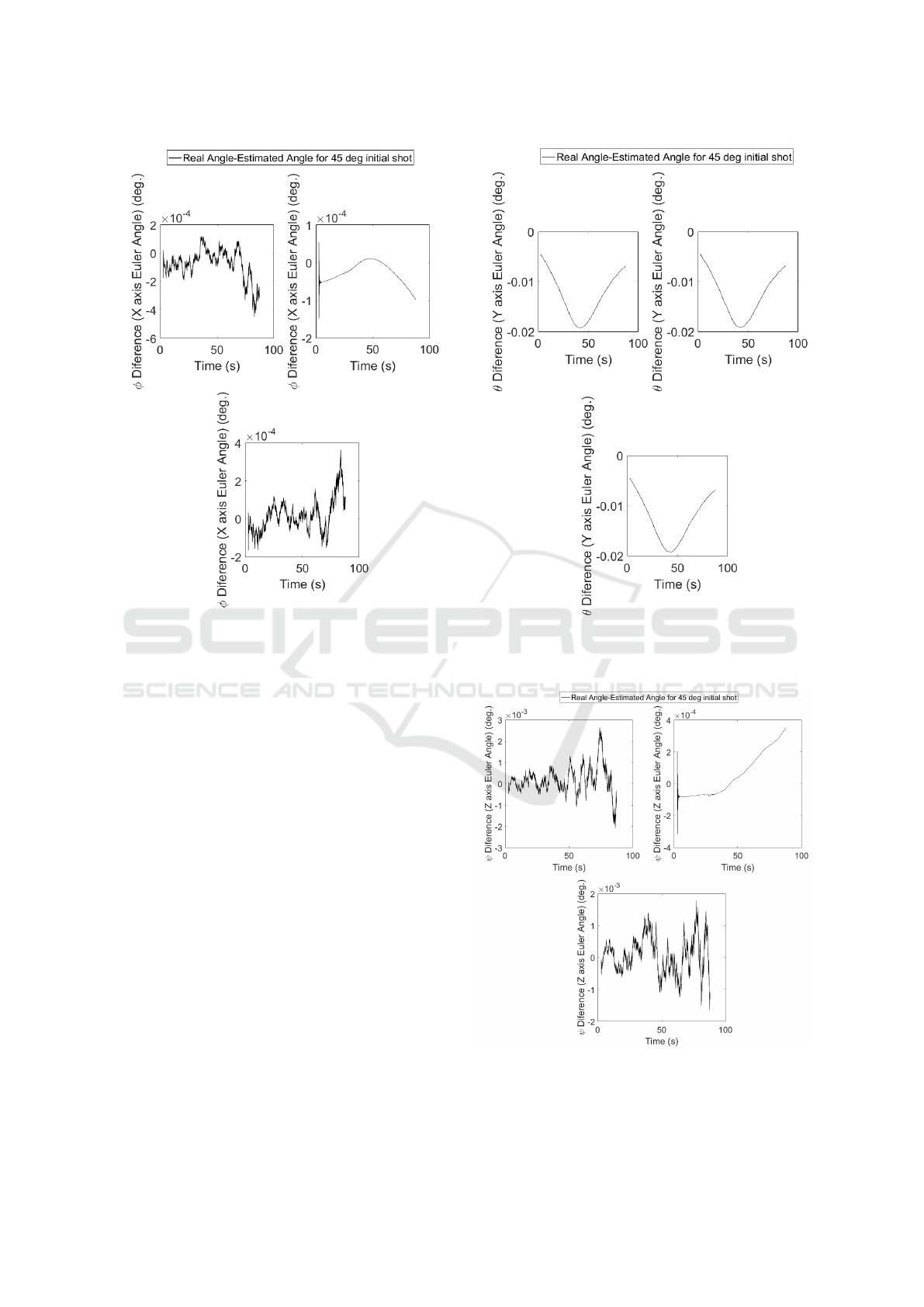
Figure 2: Comparison between estimated and real magni-

tudes for aircraft roll angle (φ) for a shot angle of 45 deg.

and azimuths of 0

◦

(left), 45

◦

(right) and 90

◦

(bottom).

However, as it is shown in the following section,

the results are accurate enough for terminal guidance

tasks in artillery.

5 SIMULATION RESULTS

Simulation results are presented using the nonlinear

ﬂight dynamics model (de Celis et al., 2017), where

data employed was validated from real ﬂights and

model accuracy tested, in order to demonstrate suit-

ability of attitude determination algorithm. A set of

ballistic simulated shots was performed as deﬁned in

the previous section, in order to compare estimated

and simulated attitudes. MATLAB/Simulink R2016a

on a desktop computer with a processor of 2.8 Ghz

and 8 GB RAM was used.

In order to compare the estimated attitude against

real or simulated attitude, the following expressions

are represented in Figures 2, 3 and 4: φ

real

−φ

estimated

real

−θ

estimated

and ψ

real

−ψ

estimated

. All these ﬁg-

ures represent results for a shot angle of 45

◦

and three

different azimuth angles: 0

◦

, 45

◦

and 90

◦

. Note that a

larger amount of simulations have been performed, as

Figure 3: Comparison between estimated and real magni-

tudes for aircraft pitch angle (θ) for a shot angle of 45 deg.

and azimuths of 0

◦

(left), 45

◦

(right) and 90

◦

(bottom).

Figure 4: Comparison between estimated and real magni-

tudes for aircraft yaw angle (ψ) for a shot angle of 45 deg.

and azimuths of 0

◦

(left), 45

◦

(right) and 90

◦

(bottom).

Aircraft Attitude Determination Algorithms Employing Gravity Vector Estimations and Velocity Measurements

381

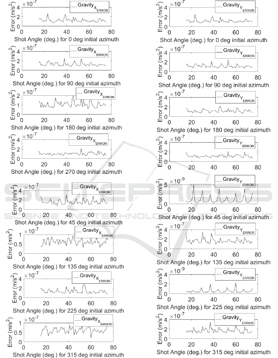
Figure 5: Representation of x

gravity component Root

Mean Squared Error along the whole trajectory for each

shot angle and for the 8 azimuths tested.

Figure 6: Representation of y

gravity component Root

Mean Squared Error along the whole trajectory for each

shot angle and for the 8 azimuths tested.

ICINCO 2017 - 14th International Conference on Informatics in Control, Automation and Robotics

382

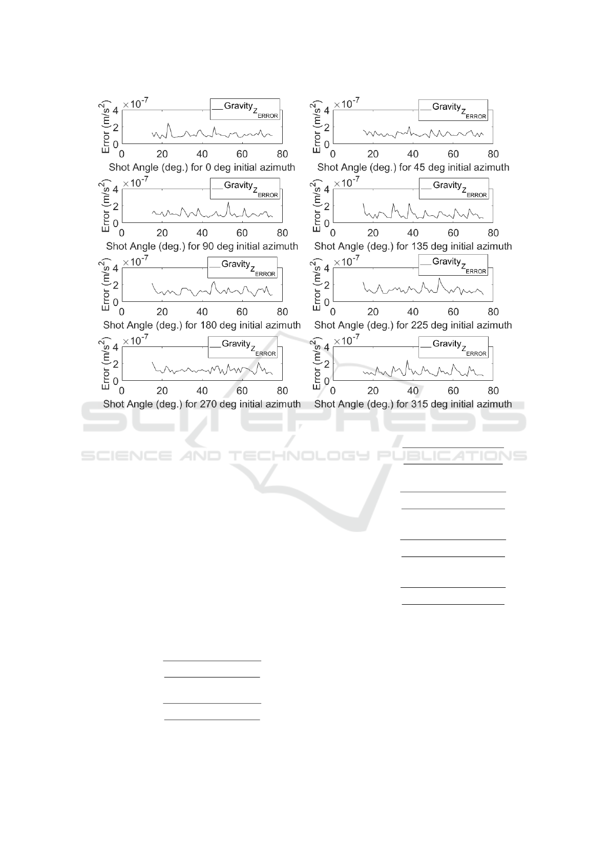
Figure 7: Representation of z

gravity component Root Mean Squared Error along the whole trajectory for each shot angle

and for the 8 azimuths tested.

it was deﬁned previously, but the results are virtually

the same.

Note that in the worst of the situations the differ-

ence between real and estimated attitude is lower than

a magnitude order of 10

−2

, which assures the appli-

cability of the presented algorithms together with the

sensors employed and their associated noises.

In order to quantify the error made in each of

the shots along the whole simulated trajectories,

the Root Mean Squared Error (RMSE) for each of

the 3 Euler angles (RMSE

,AZ

), (RMSE

,AZ

) and

(RMSE

,AZ

), and for each of the three compo-

nents of gravity vector in body axes (RMSE

,AZ

(RMSE

,AZ

) and (RMSE

,AZ

), are calculated in

(28), (29), (30),(31), (32), and (33). These errors de-

pend on the shot launch angle (θ

) and azimuth (AZ

RMSE

,AZ

(φ

real

−φ

computed

)

dσ

(28)

RMSE

,AZ

(θ

real

−θ

computed

)

dσ

(29)

RMSE

,AZ

(ψ

real

−ψ

computed

)

dσ

(30)

RMSE

,AZ

real

−g

computed

)

dσ

(31)

RMSE

,AZ

real

−g

computed

)

dσ

(32)

RMSE

,AZ

real

−g

computed

)

dσ

(33)

The computed components of gravity vector,

computed

, g

computed

and g

computed

are obtained in the

reality directly from inertial measurement unit sen-

sors, concretely by accelerometers with its associ-

ated error. On simulations performed these g

computed

and g

computed

are estimated through the fol-

lowing algorithms that take in account previously cal-

culated director cosine matrix on (14) and the errors

of accelerometers. The model of gravity vector esti-

mator is described by (34) on where

−→

acc

is the error

Aircraft Attitude Determination Algorithms Employing Gravity Vector Estimations and Velocity Measurements

383

Table 1: Representation of quadratic errors along the whole trajectory for a set of shot angles and for the 8 azimuths tested

and calculation of a representative mean parameter.

Azimuth AZ

(deg)

Shot Angle (deg.) 0 45 90 135 180 225 270 315 Total

15 QE

,AZ

7.69E-07 1.01E-07 1.00E-06 1.93E-06 1.10E-06 3.92E-07 1.30E-06 9.77E-07 3.82E-07

15 QE

,AZ

2.32E-04 2.29E-04 2.24E-04 2.21E-04 2.19E-04 2.17E-04 2.12E-04 2.09E-04 7.80E-05

15 QE

,AZ

7.69E-06 6.84E-07 6.49E-06 9.87E-06 8.16E-06 9.29E-07 4.58E-06 1.01E-05 2.46E-06

30 QE

,AZ

3.24E-06 2.38E-06 1.05E-06 2.33E-06 1.05E-06 3.52E-07 6.13E-07 1.62E-06 6.48E-07

30 QE

,AZ

1.46E-04 1.50E-04 2.31E-04 2.28E-04 2.27E-04 2.24E-04 2.21E-04 2.16E-04 7.36E-05

30 QE

,AZ

1.44E-05 6.29E-06 7.72E-06 1.25E-05 7.41E-06 1.17E-06 6.60E-06 1.54E-05 3.53E-06

45 QE

,AZ

2.45E-06 1.78E-06 2.04E-06 3.91E-06 9.67E-07 3.04E-07 7.51E-07 1.44E-06 7.10E-07

45 QE

,AZ

1.40E-04 1.43E-04 1.46E-04 1.50E-04 2.32E-04 2.32E-04 2.28E-04 2.24E-04 6.77E-05

45 QE

,AZ

1.10E-05 4.14E-06 1.41E-05 2.08E-05 1.12E-05 9.04E-07 6.63E-06 1.50E-05 4.26E-06

60 QE

,AZ

2.55E-06 1.43E-06 1.69E-06 2.05E-06 3.02E-06 2.03E-06 9.50E-07 1.66E-06 7.13E-07

60 QE

,AZ

1.36E-04 1.38E-04 1.41E-04 1.43E-04 1.46E-04 1.49E-04 2.34E-04 2.31E-04 5.98E-05

60 QE

,AZ

1.14E-05 3.02E-06 1.29E-05 1.67E-05 1.52E-05 5.60E-06 7.26E-06 1.44E-05 4.16E-06

75 QE

,AZ

1.46E-06 1.20E-06 1.27E-06 2.56E-06 2.78E-06 1.56E-06 1.66E-06 3.72E-06 7.76E-07

75 QE

,AZ

1.33E-04 1.35E-04 1.36E-04 1.38E-04 1.40E-04 1.43E-04 1.46E-04 1.49E-04 4.95E-05

75 QE

,AZ

1.10E-05 2.47E-06 9.40E-06 1.45E-05 1.40E-05 4.04E-06 1.46E-05 1.75E-05 4.25E-06

Total QE

,AZ

1.01E-06 7.02E-07 6.55E-07 1.19E-06 8.96E-07 5.27E-07 5.02E-07 9.42E-07 2.95E-07

Total QE

,AZ

7.24E-05 7.29E-05 8.09E-05 8.08E-05 8.81E-05 8.80E-05 9.42E-05 9.29E-05 2.97E-05

Total QE

,AZ

5.05E-06 1.70E-06 4.72E-06 6.85E-06 5.19E-06 1.42E-06 3.87E-06 6.57E-06 1.70E-06

associated to the accelerometer:





computed









+ q

−q

2(q

+ q

) 2(q

−q

)

2(q

−q

) q

−q

+ q

−q

2(q

+ q

)

2(q

+ q

) 2(q

−q

) q

−q

+ q









9.81





−→

acc

(34)

Table 1 shows the Root Mean Squared Errors for

the 3 Euler angles for different shot angles and az-

imuths. The ﬁrst column shows the shot angle and

the second one the displayed error (RMSE

,AZ

(RMSE

,AZ

and RMSE

,AZ

). The rest of the

columns show the numerical values of the errors for

different azimuths. Finally right column named to-

tal, represents the Root Mean Squared Errors for the

set of azimuths represented on the same row. Equally

the last three rows represent the Root Mean Squared

Errors for the set of shot angles represented on the

same column. Finally the three values of the bottom-

right corner can be considered as an estimation of the

whole error of the attitude calculation algorithms.

Figures 5, 6 and 7 show the following Root

Mean Squared Errors: RMSE

,AZ

, RMSE

,AZ

and

RMSE

,AZ

along the whole trajectory for each shot

angle and for the 8 azimuths.

Note that the obtained Root Mean Squared Errors

for all the measures of interest presented in this paper

are small enough to consider the proposed algorithm

for estimating attitude of high dynamic vehicles at a

low cost. Comparison between real aircraft attitude,

which can be assumed near to the attitude provided

by a precise gyroscope, and the attitude obtained by

exposed algorithms, never differ from 10

−3

degrees,

which is a very accurate value for most of the projec-

tile applications.

6 CONCLUSIONS

A novel low-cost approach for estimating attitude of

aerial platforms has been proposed. This approach is

based on the measurement of two different vectors:

speed and gravity vector. They are measured in two

different reference frames using a GNSS sensor and a

set of accelerometers. The presented algorithm is of

special interest for high dynamic vehicles where other

low-cost approaches, such as the ones using magne-

tometers, are not suitable.

Nonlinear simulations based on ballistic rocket

launches are performed to obtain ideal attitude and

compare it to the attitude obtained by the proposed

approach. Computational results show that errors

made are small enough to consider the presented al-

gorithm as a good candidate for using it within a con-

trol algorithm. Note that the low-cost needed compo-

nents make this approach highly interesting for non-

re-usable vehicles.

ICINCO 2017 - 14th International Conference on Informatics in Control, Automation and Robotics

384

REFERENCES

Crassidis, J. L., Markley, F. L., and Cheng, Y. (2007). Sur-

vey of nonlinear attitude estimation methods. Journal

of guidance, control, and dynamics, 30(1):12–28.

de Celis, R., Cadarso, L., and S

anchez, J. (2017). Guid-

ance and control for high dynamic rotating ar-

tillery rockets. Aerospace Science and Technology.

http://dx.doi.org/10.1016/j.ast.2017.01.026.

Eure, K. W., Quach, C. C., Vazquez, S. L., Hogge,

E. F., and Hill, B. L. (2013). An application

of uav attitude estimation using a low-cost iner-

tial navigation system. NASA/TM2013-218144.

https://ntrs.nasa.gov/archive/nasa/casi.ntrs.nasa.gov/

20140002398.pdf.

Gebre-Egziabher, D., Elkaim, G. H., Powell, J., and Parkin-

son, B. W. (2000). A gyro-free quaternion-based at-

titude determination system suitable for implementa-

tion using low cost sensors. In Position Location and

Navigation Symposium, IEEE 2000, pages 185–192.

IEEE.

Gebre-Egziabher, D., Hayward, R. C., and Powell, J. D.

(1998). A low-cost gps/inertial attitude heading ref-

erence system (ahrs) for general aviation applica-

tions. In Position Location and Navigation Sympo-

sium, IEEE 1998, pages 518–525. IEEE.

Henkel, P. and Iafrancesco, M. (2014). Tightly coupled po-

sition and attitude determination with two low-cost

gnss receivers. In Wireless Communications Sys-

tems (ISWCS), 2014 11th International Symposium

on, pages 895–900. IEEE.

Ismail, A., Ashraf, K., Metawea, A., Mostfa, I., Saeed,

A., Helal, E., Essawy, M., Abdelazim, M., Ibrahim,

M., Raafat, R., et al. (2015). A high-performance

self-clocked digital-output quartz gyroscope. In SEN-

SORS, 2015 IEEE, pages 1–4. IEEE.

Kuipers, J. B. et al. (1999). Quaternions and rotation

sequences, volume 66. Princeton university press

Princeton.

Ma, D.-M., Shiau, J.-K., Wang, I., Lin, Y.-H., et al. (2011).

Attitude determination using a mems-based ﬂight in-

formation measurement unit. Sensors, 12(1):1–23.

Mizell, D. (2003). Using gravity to estimate accelerome-

ter orientation. In Proc. 7th IEEE Int. Symposium on

Wearable Computers (ISWC 2003), volume 252. Cite-

seer.

Savage, P. G. (2000). Strapdown analytics, volume 2. Strap-

down Associates Maple Plain, MN.

Springmann, J. C. and Cutler, J. W. (2014). Flight results of

a low-cost attitude determination system. Acta Astro-

nautica, 99:201–214.

Yun, X., Bachmann, E. R., and McGhee, R. B. (2008). A

simpliﬁed quaternion-based algorithm for orientation

estimation from earth gravity and magnetic ﬁeld mea-

surements. IEEE Transactions on instrumentation and

measurement, 57(3):638–650.

Aircraft Attitude Determination Algorithms Employing Gravity Vector Estimations and Velocity Measurements

385