Cartographic Scale and Minimum Mapping Unit Influence on LULC
Modelling
David García Álvarez
Departamento de Análisis Geográfico Regional y Geografía Física, Universidad de Granada, Granada, Spain
Keywords: Scale, Minimum Mapping Unit, CORINE, SIOSE, LULC Modelling, Dinamica Ego.
Abstract: Two models at two different scales (1:25.000 and 1.100.000) were calibrated using two different Land Use
and Land Cover maps at such cartographic scales (SIOSE and CORINE) and with a different Minimum
Mapping Unit (0.2-0.5ha and 25ha). Differences between models were assessed through cross-tabulation
analysis (quantity and allocation disagreement) and spatial metrics (pattern disagreement). The models
results have been very different depending on the scale considered, although most of the disagreement
comes from the contrasting input maps. In any case, the scale at which the models were calibrated have
proved to influence the pattern modelled and the quantity and allocation of changes.
1 INTRODUCTION
Depending on the considered scale, spatial data can
offer different information about the studied features
and the relationship between them. In consequence,
scale influences any analysis of geographical data,
including Land Use and Land Cover (LULC)
modelling.
Usually scale is understood as cartographic scale
(ratio), extent (map size or study are size) or grain,
which is sometimes referred as spatial scale
(O’Sullivan and Perry, 2013). The temporal and
thematic resolution are also considered part of the
concept of scale, together with the Minimum
Mapping Unit (MMU) (Castilla et al., 2009), that is,
the smallest size area unit to be mapped. A smaller
MMU means a more detailed map, whereas a bigger
MMU reduces such detail. In the last case, smaller
features are not drawn and, consequently, the map
representation only focus on the dominant features.
Several papers have addressed the scale
influence on LULC modelling, focusing on the grain
or spatial resolution (Blanchard, Pontius Jr. and
Urban, 2015), extent (Verburg A. Veldkamp, 2004),
temporal resolution (Rosa et al., 2015) and, in the
case of CA models, neighbourhood size (Pan et al.,
2010). However, there is a lack of research about
how the cartographic scale and the Minimum
Mapping Unit (MMU) of the data vary the model
results.
Several studies proved the MMU influence on
pattern analysis and landscape metrics calculation
(Saura, 2004; Kelly, Tuxen and Stralberg, 2011).
This shows how MMU affects GIS analysis and,
therefore, the need to evaluate this component of
scale.
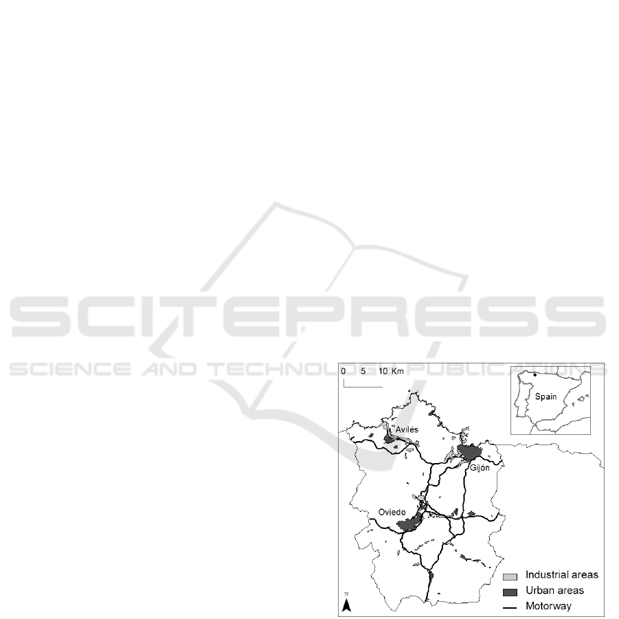
Figure 1: Asturias Central Area location. Sources:
National Topographic Map 1:200.00.
The objetive of this paper is to study the effects
of cartographic scale and MMU on LULC modelling
through the comparison of two models calibrated at
two different scales (1:100.000 and 1:25.000). We
study the quantity and allocation disagreements as
Álvarez, D.
Cartographic Scale and Minimum Mapping Unit Influence on LULC Modelling.
DOI: 10.5220/0006383003270334
In Proceedings of the 3rd International Conference on Geographical Information Systems Theory, Applications and Management (GISTAM 2017), pages 327-334
ISBN: 978-989-758-252-3
Copyright © 2017 by SCITEPRESS – Science and Technology Publications, Lda. All rights reserved
327
well as the pattern disagreement consequence of the
dissimilar data used in the scenarios generated by
the models. From this point forward, when referring
to scale we refer to the cartographic scale and
MMU.
2 STUDY AREA AND DATA SETS
2.1 Study Area
The test area was the Asturias Central Area, the
most dynamic space of Asturias (Spain) (Fig. 1).
The main changes are from rural covers to urban and
industrial spaces.
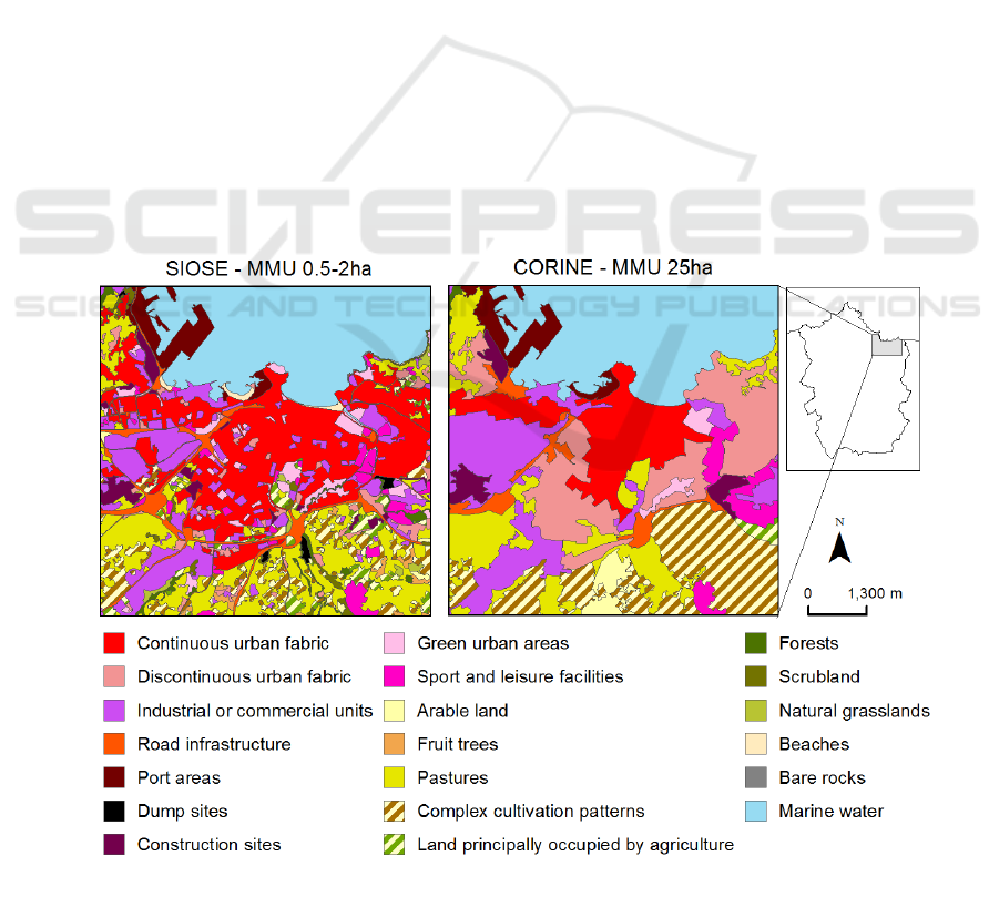
2.2 Data Sets
Two LULC maps at two cartographic scales and
with different MMU were employed: CORINE
(1:100.000; 25ha) and SIOSE (1:25.000; 0.5-2ha)
(Fig. 2).
Whereas SIOSE was obtained by photo-
interpretation of aerial imagery, CORINE was made
from a generalization of SIOSE. Therefore, both
maps refer to the same base dates (2005 and 2011)
and the differences between them are a result of the
generalization process, that is a result of the different
scale rules (MMU).
There is not a final land cover map for SIOSE.
Its data base gives information about the proportions
of every cover that compose every polygon, but
there is not a unique label that identifies all
polygons. Therefore, we carried out a generalization
of that statistical information in a way that the
geometry (polygons) is defined by a unique cover
(label). This was made through the implementation
of translation rules according to the proposal of
Delgado Hernández (2016).
To make comparable the two maps, they were
reclassified according to the same legend. Although
coarser scales usually tie in with simpler thematic
resolutions, since our objective is to analyse the
influence of cartographic scale and MMU on LULC
modelling, we have kept the thematic resolution
constant. Otherwise, the results would show the
general influence of all components of scale on
LULC models. Moreover, both map cartographic
scales (1:25.000 and 1:100.000) are regional.
Accordingly, both fit well with the proposed legend.
Finally, both data sets were rasterized at 12.5m
(SIOSE) and 50m (CORINE) following the criteria
proposed by Hengl (2006) in the search for the
Figure 2: Input maps comparison for an example area (Gijón). Sources: SIOSE (2011) and CORINE (2012)
GAMOLCS 2017 - International Workshop on Geomatic Approaches for Modelling Land Change Scenarios
328

minimum influence of the rasterization on our
analysis. That is why we have not used the reference
CORINE resolution (100m).
3 METHODS
3.1 Model Calibration and Simulation
Two models were implemented in Dinamica EGO,
one for SIOSE (1:25.000 model) and another one for
CORINE (1:100.000 model). Dinamica is a
recognized stochastic cellular automata model,
which is in addition very flexible (Mas et al., 2014).
This allowed to set up both models according to the
same criteria.
Two functions compose Dinamica EGO:
expander and patcher. The expander function models
new pixels as an expansion of previous patches,
whereas the patcher function models new pixels as a
new patch, isolated from previous patches of the
same class. More information about these functions
and the model architecture can be found in Soares,
Cerqueira and Pennachin (2002).
Dinamica Ego models transitions. Therefore,
different transitions were selected for each model
according to the changes measured by each pair of
input maps (Table 1). Only those transitions with a
minimum quantity of changes (>10ha) were
considered. Like the modelling objective is to study
how artificial surfaces expand, there were selected
only those transitions which transition to an artificial
cover.
Drivers were chosen according to expert criteria
(interviews) and literature review. When a
correlation greater than 0.5 between two drivers was
detected, one of them was removed from the model.
The driving forces included in the model are:
roads, train stations, residential and industrial
buildings, coastline, leisure facilities, population
density, slopes, planning, substratum and industrial
ports. When possible, drivers were obtained from
sources with similar scales to the implemented
models (1:25.000 and 1:100.000).
Driving forces relation with changes was
calibrated through the Weights of Evidence method,
which is part of Dinamica EGO. The two models
were run with the same weights of evidence,
according to expert criteria. This is possible because
Dinamica allows the user to modify manually the
obtained weights.
The model parameters (size and variance of new
patches) were established according to real changes
(2005-2011). Finally, when some strange or
incorrect behaviour was detected, it was corrected
manually. Thus, it was applied a manual and expert
calibration.
Once the model was calibrated, a simulation was
run to the year 2020, which fits well with the short
calibration period (six years). Transition rates for the
simulation year (2020) are a modification of the
rates of change for the calibration period according
to real trends of change for the modelled period, as
pointed out by experts.
Table 1: In grey, transitions modelled by the two models.
In white, transitions modelled by only one.
From To
Construction sites
Continuous urban
fabric
Pastures
Construction sites
Discontinuous urban
fabric
Pastures
Construction sites
Industrial and
commercial units
Arable lands
Pastures
Complex cultivation patterns
Land principally occupied by
agriculture
Forests
Natural grasslands
Scrubland
Construction sites Infrastructures
Forests
Mineral extraction
sites
Scrubland
Arable land
Pastures
Dump sites
Forests
Dump sites
Construction sites
Arable land
Pastures
Complex cultivation patterns
Land principally occupied by
agriculture
Forests
Natural grasslands
Scrubland
3.2 Data Analysis and Assessment
Disagreements were calculated for the input maps
and for the changes simulated, that is without
considering the permanent areas. Disagreements for
input maps give us information about how the
difference of the initial data can explain the results
generated by the models.
Quantity and allocation disagreements were
analysed through the matrix proposed by Pontius Jr.
and Millones (2011). For the pattern disagreement, a
series of spatial metrics were calculated through
FRAGSTATS 4.2. These are: Number of Patches
Cartographic Scale and Minimum Mapping Unit Influence on LULC Modelling
329
(NP), Area-Weighted Mean Patch Area (AWMPA)
and Patch Cohesion Index (PCI). Their selection was
based in how much information they provided, that
is how well they express the difference between the
compared maps.
4 RESULTS
4.1 Quantity and Allocation
Disagreement
There is an important difference in the quantity and
allocation of classes between the two input maps
(SIOSE and CORINE) because of their different
scale. Only around the 44% of the area in one map
corresponds to the same category in the other map
(Fig. 3).
In consequence, each map measures different
types and quantity of changes. This has resulted in
the consideration of different transitions for the two
models (Table 1). Also, like the areas where every
class is located are different (25% allocation
disagreement), the simulated changes will locate in a
different position. Since there are two models which
simulate different transitions and the location of the
classes where the transition takes place are probably
different, there is a low probability that the changes
simulated by both models would be similar.
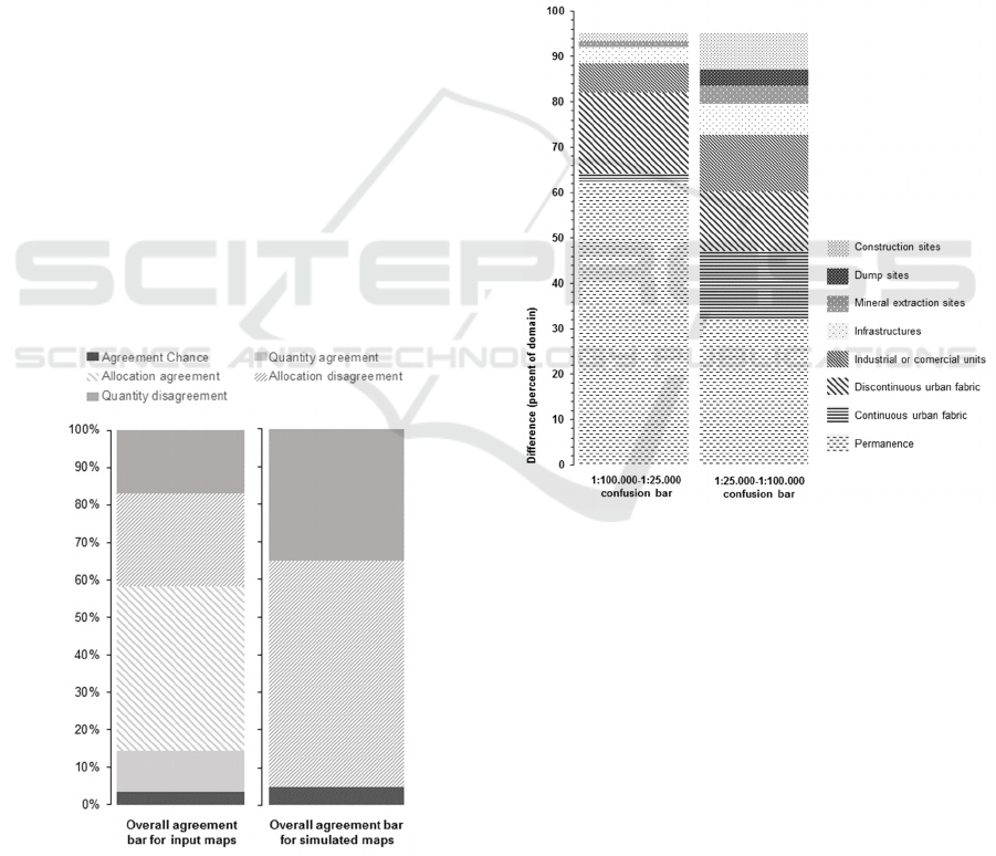
Figure 3: Overall agreement bars for input and simulated
maps.
This is what Figure 3 tell us: the only agreement
between simulated changes by the two models is due
to chance. Depending on the input maps used, the
model produces a very different result. The 95% of
the changes simulated by the two models are
different (Fig. 4)
Figure 4 allows to see the quantity disagreement
between the simulated changes depending on the
class considered. Each confusion bar is composed by
various sections, which represent the proportion of
pixels that are allocated to a different class on the
other simulation. When the section for any particular
class (e.g. continuous urban fabric) is larger in one
bar than on the other, there is a quantity
disagreement, which is proportional to the difference
between the two sections in both bars.
Figure 4: The first bar depicts the simulated areas in the
1:100.000 model that are not the same in the 1:25.000
model. The second bar depicts the simulated areas in the
1:25.000 model that are not the same in the 1:100.000
model.
The simulated changes are greater in the
1:25.000 model than in the 1:100.000 model: the
size of the confusion bar for permanence is greater
in the 1:100.000 model than in the 1:25.000 model
(Fig. 4). Hence, regarding the total area simulated as
change by both models, in the 1:100.000 model only
the 38% of the area is change, whereas in the
1:25.000 model that is true for the 68% of the area.
This is because, due to the smaller MMU, SIOSE
allows to detect small changes. Whereas only
changes over 5ha are drawn in CORINE, SIOSE
represents every change bigger than 0.4ha.
GAMOLCS 2017 - International Workshop on Geomatic Approaches for Modelling Land Change Scenarios
330
The quantity disagreements at the class level are
related to the quantity disagreements between input
maps. E.g. there is more quantity disagreement for
continuous urban fabric in the 1:25.000 model than
in the 1:100.000 model because the area of the
continuous urban fabric is bigger in the input maps
of the first model (SIOSE) than in the input maps of
the second model (CORINE).
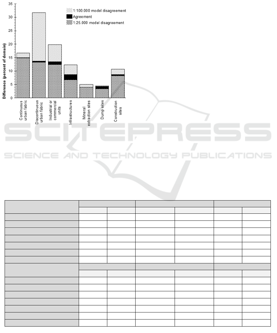
Figure 5: Agreement bars per category for simulated
changes in the two models (1:100.000 and 1:25.000).
Like the only agreement between simulated
changes is due to chance, the allocation
disagreement bars at the class level don´t give us
extra information (Fig. 5). Most of the area in the
bars are disagreements and, therefore, their
information corresponds to the disagreements
showed by Figure 4.
No allocation agreement is achieved because,
whereas the drivers are the same in the two models,
the candidate areas to transition are located in
different places. The bigger the quantity and
allocation disagreement between input maps, the
bigger the probability that a same pixel is located in
a different place in the two maps and, therefore, the
bigger the probability that the candidate pixel to
transition would be different in the two models.
4.2 Pattern Disagreement
The pattern simulated by the two models is related to
the input maps pattern. However, when one
compares real changes (2005-2011) to simulated
changes, the results show how the model behaves
similarly independent of the considered scale.
Despite of the bigger MMU for CORINE (25ha)
than for SIOSE (0.5-2ha), there are not big
differences in the fragmentation of changes for the
1:100.000 and 1:25.000 models (Table 2). In fact,
some classes show a bigger area-weighted mean
patch area (polygon mean area corrected by the
polygon size) for the model at a finer scale than for
the model at a coarser scale. Likewise, the number
of changing patches increases with the simulation
for the coarser model, whereas it falls for the finer
model.
Whereas the effect of the MMU rule is evident
for the real changes (input maps cross tabulation),
we can´t perceive it in the simulated changes (Table
Table 2: Spatial metrics at the class level for real (2005-2011) and simulated (2011-2020) changes.
Simulated changes
2011-2020
Number of pathes Area-weighted mean patch area Patch cohesion index
1:25 1:100 1:25 1:100 1:25 1:100
Continuous urban fabric 44 13 10.7344 3.3967 95.0723 71.0631
Discontinuous urban fabric 79 88 11.9334 16.5856 93.7738 80.4932
Industrial or commercial units 81 42 14.9641 8.1407 95.7527 79.9843
Infrastructures 15 4 14.5344 32.3644 96.4041 92.4082
Mineral extraction sites 35 5 1.9123 3.537 90.3935 72.052
Dump sites 11 4 7.7488 5.1667 94.9689 77.3581
Construction sites 118 26 3.3104 2.9085 90.2173 63.8639
Input maps changes
2005-2011
Number of pathes Area-weighted mean patch area Patch cohesion index
SIOSE CORINE
SIOSE CORINE
SIOSE CORINE
Continuous urban fabric 72 4 19.5006 12.5078 96.4369 86.0809
Discontinuous urban fabric 130 19 11.6396 43.5088 93.5797 92.4059
Industrial or commercial units 130 23 26.328 34.0165 95.7127 89.8172
Infrastructures 8 1 13.3087 35.75 96.6727 93.0449
Mineral extraction sites 64 2 5.3172 18.8616 92.89 88.8021
Dump sites 34 8 5.578 7.3148 93.4537 80.6492
Construction sites 95 10 37.7259 83.333 97.3597 95.4769
Cartographic Scale and Minimum Mapping Unit Influence on LULC Modelling
331

2). That is because the models work at the pixel
level, regardless of the MMU. Since the pixel size is
much smaller than the MMU (156m
2
(1:25.000) vs
0.2-0.5ha (SIOSE) and 0.25ha (1.100.000) vs 25ha
(CORINE)), there is not much difference in the
model behaviour because of the MMU.
The bigger the contrast between the MMU and
the pixel size, the more evident the effects of the
model behaviour in the resultant pattern. That is the
reason why the 1:100.000 model show a more
contrasted behaviour regarding to real changes than
the 1:25.000 model.
Like there are not MMU rules, the connection or
aggregation of simulated changes (patch cohesion
index) is smaller than the aggregation of real
changes in both models, although the contrast is
again more pronounced for the coarse scale model
than for the fine scale one.
5 DISCUSSION
5.1 Input Maps
Input maps play an essential role on the model
results. Therefore, knowing the uncertainty of the
data sets which we are using it is critical in
modelling research (Verburg, Neumann and Nol,
2011), since most of the model conclusions will be a
consequence of how these maps reflect reality.
The results have showed important differences
between input maps (SIOSE and CORINE). This has
been a great limitation for the models agreement: the
dissimilar quantities and allocations of the same
categories turn out on different possibilities to
allocate the same transitions.
Working with maps at lower thematic resolutions
can help to achieve a higher agreement between
input maps. Thus, uncertainty is usually lower at
coarser scales since local changes are omitted
(Verstegen et al., 2012).
5.2 Model Calibration
The finer the scale considered, the bigger the
information that input maps provide. Accordingly,
maps at finer scales (SIOSE) show a bigger quantity
and types of changes than maps at coarser scales
(CORINE). In consequence, transition rates
(estimated quantities of changes) and potential
transitions (type of changes modelled) are different
depending on the scale of the model: the quantity of
changes and the number of transitions are bigger for
the 1:25.000 model than for the 1:100.000 model.
The provision of more information about reality
can be seen as an advantage because we can
understand better the dynamics of our study area.
However, it is also a limitation when we need to
manage tons of complex information to calibrate the
model. At finer scales, transitions rarely occur alone
and different transitions happen together. The
patterns of change are also more complex.
When using fine scale maps, we also need to pay
attention to the possible noise in the data. The finer
the scale considered, the greater the possibility to
find noise (small changes that are not real changes).
This noise will influence the results of our model.
Thus, the modeller has to find a balance between
data detail and model complexity. More detail but
much more complexity is worse than less detail and
a very simple model (Wainwright and Mulligan,
2013). The perfect balance would be a manageable
complexity level which is in accordance with the
detailed added to the model.
Also, depending on the dynamics that the
modeller can explain, a finer or coarser scale should
be chosen. The 1:100.000 and 1:25.000 models were
calibrated using the same driving forces, despite of
the fact that their input maps show different
dynamics.
The SIOSE maps show small changes, because
of the small MMU, that are not correctly modelled
since there are not additional drivers to explain
them. For certain classes, like dump sites, the
1:25.000 model identifies more changes. However,
most of these new changes come from processes that
are different to the processes which cause the
changes identified by the 1:100.000 model. Like we
model in both cases the changes with the same
drivers, the 1:25.000 model extrapolates changes
from one process to changes from other processes.
If there is only information for the main
dynamics of the study area, a coarse scale model,
like the 1:100.000 model, is advisable. However, if
we can explain also the small changes which are
visible in SIOSE, the 1:25.000 model is maybe the
best option.
Nevertheless, CORINE maps only reflects the
bigger changes in the Asturias Central Area.
Because of the scarce dynamics of this area when
compared with metropolitan areas or other big cities,
the changes showed by CORINE are few and with
very specific locations. Therefore, it is difficult to
extract an organic growing pattern from that data.
Consequently, depending on the area studied and
its characteristics, most of the dynamics can only
emerge at specific scales. If the urban sprawling
comes from small urban patches, a fine scale map is
GAMOLCS 2017 - International Workshop on Geomatic Approaches for Modelling Land Change Scenarios
332

needed. However, in the opposite case, a coarse map
can be sufficient.
Therefore, every scale has some advantages and
limitations. The modeller mission is, as pointed out
previously, to find a balance between all the
requirements.
5.3 Simulations
The two scenarios generated by the two calibrated
models are very different. The agreement between
them is only by chance. Most of this difference
comes from the contrasted information in the input
maps (quantity and allocation disagreement). The
stochastic component of the model must have
influenced the results also. Nevertheless, the scale
and resolution at which the model is set up also have
played a role in the resultant scenario.
Grain is considered as spatial scale and it is
related to the others concepts of scale: small MMU
imply finer spatial resolution than larger units. Then,
models at finer scales (1:25.000, 12.5m) simulate
more pixels than models at coarser scales
(1:100.000, 50m). As a result, the quantity of pixels
to allocate is not the same for models at different
scales and resolutions: the bigger the resolution, the
bigger the quantity of pixels to allocate and the more
likely the model to make a mistake. Therefore, the
probability to make a mistake is greater for finer
scale models than for coarser scales models.
Similar studies which have focused the analysis
on the influence of the spatial resolution on LULC
modelling have reached similar conclusions
(Marceau et al., 2005; Pan et al., 2010).
In addition, there is an incoherence between the
model resolution (12.5m and 50m) and the MMU
(0.2-0.5ha and 25ha). This makes the pattern of the
simulated scenarios more fragmented than the initial
pattern, especially when we are working with maps
that have big MMU, like CORINE. The model
allocates changes as pixels whereas input maps only
show changes that meet the MMU. In consequence,
the changes allocated by the model will be smaller
than the changes measured by the input maps.
Model validation through techniques that
compare the generated scenario with the real map
for the same date are not completely reliable.
Whereas the scenario doesn´t meet with the MMU
rules, the reference map does. Consequently, they
are never going to show the same information. A
real change that only affects a pair of pixels won´t
be reflected in the reference maps because it doesn´t
comply with the minimum required size. However,
the model does can simulate correctly that change.
Dinamica EGO allows the user to achieve the
wished simulation pattern through the functions
expander and patcher. One can decide how much
pixels will be allocated as expansion of previous
patches and how much pixels will conform new
patches for every simulated category. The user can
decide also, for every transition, the mean and
variance of the new patches generated.
Although that seems a solution for the proposed
problem (Soares-Filho et al., 2003), that did not
work for our study area. The mean and variance
parameters are only considered when there is an
enough variety of candidate areas of different sizes
for a specific transition. A candidate area is possible
when inside a polygon of the destination category of
the transition there is a suitable area, that is an area
that, according to the model driving forces, has a
value above 0.
Suitable areas for transitions are going to be
smaller in models at finer scales (1:25.000) than in
models at coarser scales (1:100.000) because of the
respective size of the polygons in each model
(MMU). Therefore, models at finer scales (smaller
MMU), as far as their input maps are composed by
small polygons, find more difficult to vary the
desired pattern than models at coarser scales (bigger
MMU).
Patch-based models can be a solution for all
these problems (Wang and Marceau, 2013).
4 CONCLUSIONS
There is an important source of uncertainty
consequence of the chosen scale in LULC
modelling, as it is in any GIS analysis.
Firstly, this uncertainty comes from the input
maps dissimilarity. LULC data for the same area
offer different information depending on the
cartographic scale and minimum mapping unit
(MMU). The input maps selected, as far as they
show a specific representation of a given area, will
provide different input parameters to the LULC
model.
Making these maps simpler (e.g. decreasing
thematic resolution) can reduce the dissimilarity
between them at the expense of model complexity.
Secondly, uncertainty comes from the scale at
which the model is set up. Modelled patterns are
dependent on the spatial resolution, which is linked
with the MMU: small MMU imply finer spatial
resolution than larger units. The quantity and detail
of changes also vary with the scale. Models at finer
scales manage more information than models at
Cartographic Scale and Minimum Mapping Unit Influence on LULC Modelling
333

coarser scales, although they are more complex to
calibrate since the greater the quantity of
information, the higher the model complexity. How
the modeller manages this complexity can introduce
additional uncertainty in the model. Therefore, the
user must strike a balance between model
complexity and explanatory power.
ACKNOWLEDGEMENTS
This work has been supported in part by project
SIGEOMOD_2020. BIA2013-43462-P (Spanish
Ministry of Economy and Competitiveness and the
Feder European Regional Development Fund). The
author is also grateful to the Spanish Ministry of
Economy and Competitiveness and the European
Social Fund for the funding of his research activity
(Ayudas para contratos pre-doctorales para la
formación de doctores 2014).
REFERENCES
Blanchard, S. D., Pontius Jr., R. G. and Urban, K. M.
(2015) ‘Implications of Using 2 m versus 30 m Spatial
Resolution Data for Suburban Residential Land
Change Modeling’, Journal of Environmental
Informatics, 25(1), pp. 1–13. doi:
10.3808/jei.201400284.
Castilla, G., Larkin, K., Linke, J. and Hay, G. J. (2009)
‘The impact of thematic resolution on the patch-
mosaic model of natural landscapes’, Landscape
Ecology, 24(1), pp. 15–23. doi: 10.1007/s10980-008-
9310-z.
Delgado Hernández, J. (2016) Methodology of
classification extraction from descriptive systems of
land cover and land use. doi:
10.13140/RG.2.1.2639.5921.
Hengl, T. (2006) ‘Finding the right pixel size’, Computers
and Geosciences, 32(9), pp. 1283–1298. doi:
10.1016/j.cageo.2005.11.008.
Kelly, M., Tuxen, K. A. and Stralberg, D. (2011)
‘Mapping changes to vegetation pattern in a restoring
wetland: Finding pattern metrics that are consistent
across spatial scale and time’, Ecological Indicators.
Elsevier Ltd, 11(2), pp. 263–273. doi:
10.1016/j.ecolind.2010.05.003.
Marceau, D. J., others, Ménard, A. and Marceau, D. J.
(2005) ‘Exploration of spatial scale sensitivity in
geographic cellular automata’, Environment and
Planning B: Planning and Design, 32(5), pp. 693–714.
doi: 10.1068/b31163.
Mas, J.-F., Kolb, M., Paegelow, M., Camacho Olmedo, M.
T. and Houet, T. (2014) ‘Inductive pattern-based land
use/cover change models: A comparison of four
software packages’, Environmental Modelling &
Software, 51, pp. 94–111. doi:
10.1016/j.envsoft.2013.09.010.
O’Sullivan, D. and Perry, G. L. W. (2013) Spatial
Simulation: Exploring Pattern and Process.
Chichester: John Wiley & Sons.
Pan, Y., Roth, A., Yu, Z. and Doluschitz Reiner, R. (2010)
‘The impact of variation in scale on the behavior of a
cellular automata used for land use change modeling’,
Computers, Environment and Urban Systems, 34(5),
pp. 400–408. doi:
10.1016/j.compenvurbsys.2010.03.003.
Pontius Jr., R. G. and Millones, M. (2011) ‘Death to
Kappa: birth of quantity disagreement and allocation
disagreement for accuracy assessment’, International
Journal of Remote Sensing, 32(15), pp. 4407–4429.
doi: 10.1080/01431161.2011.552923.
Rosa, I. M. D., Purves, D., Carreiras, J. M. B. and Ewers,
R. M. (2015) ‘Modelling land cover change in the
Brazilian Amazon: temporal changes in drivers and
calibration issues’, Regional Environmental Change,
15(1), pp. 123–137. doi: 10.1007/s10113-014-0614-z.
Saura, S. (2004) ‘Effects of remote sensor spatial
resolution and data aggregation on selected
fragmentation indices’, Landscape Ecology, 19(2), pp.
197–209. doi:
10.1023/B:LAND.0000021724.60785.65.
Soares, B. S., Cerqueira, G. C. and Pennachin, C. L.
(2002) ‘DINAMICA - a stochastic cellular automata
model designed to simulate the landscape dynamics in
an Amazonian colonization frontier’, Ecological
Modelling, 154(3), pp. 217–235. doi: 10.1016/S0304-
3800(02)00059-5.
Soares-Filho, B. S., Corradi Filho, L., Coutinho Cerqueira,
G. and Leite Araujo, W. (2003) ‘Simulating the spatial
patterns of change through the use of the dinamica
model’, in Anais XI SBSR
, pp. 721–728.
Verburg, P. H., Neumann, K. and Nol, L. (2011)
‘Challenges in using land use and land cover data for
global change studies’, Global Change Biology, 17(2),
pp. 974–989. doi: 10.1111/j.1365-2486.2010.02307.x.
Verburg A. Veldkamp, H. P. (2004) ‘Projecting landuse
transitions at forest in the Philippines at two spatial
scales’, Landscape Ecology, 19, pp. 77–98. doi:
10.1023/B:LAND.0000018370.57457.58.
Verstegen, J. A., Karssenberg, D., van der Hilst, F. and
Faaij, A. (2012) ‘Spatio-temporal uncertainty in
Spatial Decision Support Systems: A case study of
changing land availability for bioenergy crops in
Mozambique’, Computers, Environment and Urban
Systems, 36(1), pp. 30–42. doi:
10.1016/j.compenvurbsys.2011.08.003.
Wainwright, J. and Mulligan, M. (2013) Environmental
Modelling: Finding Simplicity in Complexity. Second
edi. Edited by J. Wainwright and M. Mulligan. John
Wiley & Sons.
Wang, F. and Marceau, D. J. (2013) ‘A patch-based
cellular automaton for simulating land-use changes at
fine spatial resolution’, Transactions in GIS, 17(6), pp.
828–846. doi: 10.1111/tgis.12009.
GAMOLCS 2017 - International Workshop on Geomatic Approaches for Modelling Land Change Scenarios
334
