Three-phase Optimal Power Flow for Smart Grids by Iterative

Nonsmooth Optimization

Y. Shi

, H.D. Tuan

and A.V. Savkin

Faculty of Engineering and Information Technology, University of Technology Sydney,

2007, Sydney, NSW, Australia

School of Electrical Engineering and Telecommunications, The University of New South Wales,

2052, Sydney, NSW, Australia

Keywords:

Three-phase Optimal Power Flow (TOPF), Smart Grids, Rank-one Matrix Constraint, Nonsmooth Optimiza-

tion, Semi-deﬁnite Programming (SDP).

Abstract:

Optimal power ﬂow is important for operation and planning of smart grids. The paper considers the so called

unbalanced thee-phase optimal power ﬂow problem (TOPF) for smart grids, which involves multiple quadratic

equality and indeﬁnite quadratic inequality constraints to model the bus interconnections, hardware capacity

and balance between power demand and supply. The existing Newton search based or interior point algorithms

are often trapped by a local optimum while semideﬁnite programming relaxation (SDR) even fails to locate a

feasible point. Following our previously developed nonsmooth optimization approach, computational solution

for TOPF is provided. Namely, an iterative procedure for generating a sequence of improved points that

converges to an optimal solution, is developed. Simulations for TOPF in unbalanced distributed networks are

provided to demonstrate the practicability and efﬁciency of our approach.

1 INTRODUCTION

Optimal power ﬂow (OPF) for minimizing the cost of

power generation subject to operating constraints and

meeting demands provides one of the most important

applications of smart grids (Farhangi, 2010).

There are two types of modeling distribution net-

works in smart grid: balanced equivalent single-phase

modelling, which aims at naively approximating the

network by a balanced system of three decoupled

single-phase subsystems, and unbalanced three-phase

modelling, which preserves the unbalanced structure

of the network for constructive power ﬂow analysis

(Yang and Li, 2016). In recent years, more attentions

have been paid to the unbalanced three-phase model-

ling (Kersting, 2007).

The single-phase OPF problem in balanced trans-

mission networks has been more or less well studied

(see e.g. (Lavaei and Low, 2012; Bukhsh et al., 2013;

Madani et al., 2015)). However, the unbalanced three-

phase optimal power ﬂow problem (TOPF) in unba-

lanced networks is still left open with no available ef-

ﬁcient computational solution due its nonlinearity.

The nonlinear power balance equality constraints

of TOPF have been linearized in (Deshmukh et al.,

2012) using the ﬁrst-order Taylor expansion. As

a result, its found solution is not necessarily feasi-

ble for TOPF. On the other hand, (Abdelaziz et al.,

2013) proposed to combine Newton-Raphson met-

hod and trust region method to handle these nonli-

near constraints, which may lead to a local optimum

only. Furthermore, (Dall’Anese et al., 2013) em-

ployed semi-deﬁnite programming relaxation (SDR)

to address the TOPF. Namely, TOPF is equivalently

expressed by a convex semi-deﬁnite program (SDP)

with the additional nonconvex matrix rank-one con-

straint. The latter is then dropped for SDR. It has been

claimed in (Dall’Anese et al., 2013) that the optimal

solution of SDR is always turned-out to be rank-one

so it provides the global optimal solution of TOPF.

However, our simulation will show that it is not quite

the case, i.e. the optimal solution of SDR is turned

out to be high rank and as such it cannot provide even

a feasible point for TOPF.

In this paper, we follow the approach of (Phan

et al., 2012; Shi et al., 2015) to provide computati-

onal solution for TOPF. Namely, we develop an efﬁ-

cient iterative procedure, which invokes a SDP in each

iteration to generate a sequence of infeasible points,

which quickly converges to the optimal solution of

Shi, Y., Tuan, H. and Savkin, A.

Three-phase Optimal Power Flow for Smart Grids by Iterative Nonsmooth Optimization.

DOI: 10.5220/0006365803230328

In Proceedings of the 6th International Conference on Smart Cities and Green ICT Systems (SMARTGREENS 2017), pages 323-328

ISBN: 978-989-758-241-7

323

TOPF.

The paper is structured as follows. Section II is

devoted to the TOPF model formulation for smart

grids. Section III provides the equivalent matrix opti-

mization formulation. A nonsmooth optimization al-

gorithm for its solution is developed in Section IV.

Section V provides simulation to show the efﬁciency

of our methods. The conclusions are drawn in Section

VI.

The notations used in this paper are standard. Par-

ticularly, j denotes the imaginary unit, (X)

∗

means

element wise complex conjugate operation of vec-

tor/matrix X, M  0 means the Hermitian symme-

tric matrix M is positive semi-deﬁnite, rank(M) and

Tr(M) are the rank and trace of matrix M, respecti-

vely; ℜ(·) and ℑ(·) denote the real and imaginary

parts of a complex quantity. a ≤ b for two complex

numbers a and b is componentwise understood, i.e.

ℜ(a) ≤ ℜ(b) and ℑ(a) ≤ ℑ(b).

2 TOPF STATEMENT

Consider a three-phase network with a set of nodes

N := {1,2,· ·· ,n}. The nodes are connected through

a set of ﬂow lines L ⊆ N × N , i.e. node k is con-

nected to node m if and only if (k, m) ∈ L. Accor-

dingly, N (k) is the set of other nodes connected to

node k. A subset G ⊆ N of nodes is supposed to be

connected to generators. Any node k ∈ N \ G is thus

not connected to generators. Denote by φ ∈ {a,b,c}

the node phase. Accordingly V

and I

are the com-

plex voltage and current at node k on phase φ.

Practically, all loads in smart grids are assumed

constant, while the reactance between the neutral po-

tentials and ground is assumed to be zero. Fig.1 de-

picts the π−equivalent model is used for this three-

phase unbalanced network, which involves both self-

impedance and mutual-impedance with other phase.

Other forms of load models can be easily incorpora-

ted by introducing additional linear terms in the for-

mulation.

Figure 1: Three-phase distributed line model.

Let V

= [V

]

be the three-phase complex

voltage injected to node k ∈ N , I

= [I

]

be the three-phase complex current in the power line

(k, m) ∈ L, and y

∈ C

3×3

be three-phase admittance

of line (k, m). Then,





















−V





(1)

Other notations are:

• S

= [S

]

is three-phase apparent po-

wer transferred from node k to node m, S

+ jQ

, where P

and Q

represent three-

phase real and reactive line power, respectively;

• S

= [S

]

is three-phase apparent po-

wer injected by node k ∈ G, S

= P

+ jQ

where P

and Q

represent three-phase real and

reactive generated power, respectively;

• S

= [S

]

is three-phase apparent po-

wer injected by node k ∈ N \G, S

= P

+ jQ

where P

and Q

represent three-phase real and

reactive load power, respectively;

Let [·]

diag

denote an operator that transport an n × 1

vector to the diagonal of an n × n diagonal matrix.

Then it is obvious that,

− S

= P

− P

+ j(Q

− Q

)

= [V

]

diag

∑

m∈N (k)

∗

= [V

]

diag

∑

m∈N (k)

∗

−V

∗

)]. (2)

Therefore, we can express the three-phase real ge-

nerated power P

and reactive generated power Q

at node k as the following nonconvex quadratic functi-

ons of the node voltage V

= P

+ ℜ([V

]

diag

∑

m∈N (k)

∗

−V

∗

)]),

= Q

+ ℑ([V

]

diag

∑

m∈N (k)

∗

−V

∗

)]).

(3)

The objective of TOPF is to minimize the following

cost function of real active generated power P

f (P

) =

∑

k∈G

∑

φ∈{a,b,c}

)

+ c

), (4)

where (P

) are the real generated power on phase φ,

φ ∈ {a,b,c}, c

> 0,c

are given. Substituting

(3) in (4), the objective turns to be a function over bus

voltages V :

f (V ) =

∑

k∈G

∑

φ∈{a,b,c}

+ ℜ([V

]

diag

∑

m∈N (k)

∗

−V

∗

)])

)

+ c

+ ℜ([V

]

diag

∑

m∈N (k)

∗

−V

∗

)])

) + c

). (5)

SMARTGREENS 2017 - 6th International Conference on Smart Cities and Green ICT Systems

324

Accordingly, TOPF problem is formulated as

min

V ∈C

f (V ) s.t. (6a)

−P

− jQ

= [V

]

diag

∑

m∈N (k)

∗

−V

∗

)],∀k ∈ N \ G (6b)

min

≤ P

+ ℜ([V

]

diag

∑

m∈N (k)

∗

−V

∗

)]) ≤ P

max

,∀k ∈ G (6c)

min

≤ Q

+ ℑ([V

]

diag

∑

m∈N (k)

∗

−V

∗

)]) ≤ Q

max

,∀k ∈ G (6d)

)

min

≤ |V

| ≤ (V

)

max

,∀k ∈ N (6e)

| = |[V

]

diag

∗

−V

∗

)]| ≤ S

max

∀(k, m) ∈ L (6f)

−V

| ≤ (V

)

max

,∀(k,m) ∈ L (6g)

∀φ ∈ {a,b,c}.

where

• (6b) is the equation of the balance between the

demand and supply power at the load node k ∈

N \ G;

• (6c)-(6d) are the power generation bounds, where

)

min

, (Q

)

min

and (P

)

max

, (Q

)

max

are the

lower bound and upper bound of the real power

reactive power generations on phase φ, respecti-

vely;

• (6e) are the voltage amplitude bounds;

• (6f)-(6g) are capacity limitations, where line cur-

rents between the connected nodes are constrai-

ned by (6f), while (6g) guarantees the voltage dif-

ference in terms of their magnitude (Zimmerman

et al., 2011);

3 MATRIX RANK-ONE

CONSTRAINED

OPTIMIZATION FOR TOPF

Deﬁne

V := [V

,··· ,V

]

∈ C

and

I := [I

,··· ,I

]

∈ C

where V

and I

are the complex three-phase voltage

and current respectively. Deﬁne a symmetric block

matrix Y ∈ C

3n×3n

, with diagonal block

∑

m∈N (k)

and off-diagonal block −y

. Set y

= 0 if node k

and m are not connected. The Ohm’s law is written as

I = YV.

The voltage inserted at node k of phase φ can be

expressed by

= (e

)

V, φ ∈ a,b, c (7)

where e

= [0

1×3(k−1)

, ¯e

1×3(n−k)

]

, ¯e

denotes the

canonical basis of R

Under the deﬁnition of the outer product matrix

W = VV

, for each phase φ, constraint (6b) becomes

a linear function of W as follows,

−P

− jQ

= V

)

∗

= (V

)

YV )

= Tr(Y

W ), (8)

where Y

= e

)

Y .

Similarly, the injected real and reactive powers

corresponding to constraint (6c)and (6d) can be ex-

pressed by the following linear constraints in W :

+ ℜ(V

∑

m∈N (k)

∗

−V

∗

)]

) = (9)

+ Tr(1/2(Y

+ (Y

)

)W )

+ ℑ(V

∑

m∈N (k)

∗

−V

∗

)]

) = (10)

+ Tr( j/2(Y

− (Y

)

)W )

Constraint (6e) is also linear in W because

= (V

)

∗

= V

)

= Tr(e

)

W ) (11)

Next, deﬁne complex matrix A

and B

as,

: = [0

3×3(k−1)

3×3(m−k−1)

−y

3×3(n−m)

]

3×n

: = [0

3×3(k−1)

3×3

3×3(n−k)

]

3×n

Then, it is obvious that I

= (y

− V

))

¯e

V )

¯e

= (B

V )

¯e

, ¯e

denotes the ca-

nonical base of R

, thus, S

= V

)

∗

¯e

( ¯e

)

V = Tr(B

¯e

( ¯e

)

W ). There-

fore, the line ﬂow constraint (6f) can be re-expressed

| = |Tr(B

¯e

( ¯e

)

W )| ≤ (S

)

max

,∀(k,m) ∈ L

(12)

Three-phase Optimal Power Flow for Smart Grids by Iterative Nonsmooth Optimization

325

Similarly, the line ﬂow constraint (6g) can be re-

expressed by

−V

= V

− B

)

¯e

( ¯e

)

− B

= Tr((B

− B

)

¯e

( ¯e

)

− B

)W )

≤ (V

)

max

,∀(k,m) ∈ L

(13)

In summary, TOPF (6) is reformulated by the follo-

wing optimization problem in matrix W ∈ C

3n×3n

min

W ∈C

3n×3n

F(W ) s.t. (14a)

−P

− jQ

= Tr(Y

W ),∀k ∈ N \ G, (14b)

)

min

≤ P

+ Tr(1/2(Y

+ (Y

)

)W )

≤ (P

)

max

,∀k ∈ G (14c)

min

≤ Q

+ Tr( j/2(Y

− (Y

)

)W )

≤ Q

max

,∀k ∈ G (14d)

min

)

≤ Tr( ¯e

( ¯e

)

W ) ≤ (V

max

)

,∀k ∈ N (14e)

|Tr(B

)

W )| ≤ (S

)

max

,∀(k,m) ∈ L (14f)

Tr((B

− B

)

¯e

( ¯e

)

− B

)W )

≤ (V

max

)

,∀(k,m) ∈ L (14g)

W  0, (14h)

rank(W ) = 1, (14i)

where

F(W ) =

∑

k∈G

+ Tr(1/2(Y

+ (Y

)

)W ))

+ Tr(1/2(Y

+ (Y

)

)W ))

], (15)

which is convex quadratic in W .

As all constraints (14b)-(14h) are linear, the difﬁculty

of (14) is now concentrated at the nonconvex matrix

rank-one constraint (14i). The existing SDRs, such as

(Lavaei and Low, 2012) and (Dall’Anese et al., 2013)

simply drop the only nonconvex constraint (14i) to

have the SDP (14a)-(14h). If the optimal solution of

this SDR is of rank-one, i.e. it satisﬁes the nonconvex

rank-one constraint (14i) then it obviously leads to

the global optimal solution of the nonconvex program

(14). Otherwise, SDR cannot provide even feasible

point to the original TOPF (6). In the next section

we will provide an efﬁcient computational nonsmooth

algorithm for the optimal solution of the nonconvex

problem (14).

4 NONSMOOTH OPTIMIZATION

ALGORITHM FOR TOPF

In this section, followed by our previous work (Shi

et al., 2015), a nonsmooth optimization algorithm is

proposed to deal with the nonconvex rank-one con-

straint (14i) in program (14). Firstly, the rank-one

constraint (14i) is equivalently expressed by the fol-

lowing spectral constraint

Trace(W) − λ

max

(W ) ≤ 0, (16)

where λ

max

(W ) stands for the maximal eigenvalue of

W .

Instead of dealing with the nonconvex constraint

(16), we incorporate it into the objective, leading to

the following formulation

min

W ∈C

3n×3n

F(W )+ µ(Trace(W ) − λ

max

(W )) s.t.

(14b) − (14h), (17)

where µ > 0 is a penalty parameter. The above pe-

nalization is exact because the constraint (16) can be

satisﬁed by a minimizer of (14) with a ﬁnite value of

µ. On the other hand, any feasible W to (14) is also fe-

asible to (17), implying that the optimal value of (14)

for any µ > 0 is upper bounded by the optimal value

of (17).

Function λ

max

(W ) is nonsmooth but is lower

bounded by a linear function as the following relation

shows (Tuan et al., 2000):

max

(W ) ≥ λ

max

(κ)

) + (w

(κ)

max

)

(W −W

(κ)

max

= (w

(κ)

max

)

W w

(κ)

max

, ∀W  0. (18)

Here, w

(κ)

max

is the eigenvector corresponding to the ei-

genvalue λ

max

(κ)

Therefore, for any W

(κ)

feasible to convex con-

straints (14b)-(14h), the following SDP yields an up-

per bound for nonconvex program (17)

min

W ∈C

3n×3n

(κ)

(W ) := F(W ) + µ[Trace(W )−

(κ)

max

)

W w

(κ)

max

] s.t. (14b) − (14h)

(19)

because

(κ)

(W ) ≥ F(W )+µ(Trace(W )−λ

max

(W )) ∀ W  0

according to (18).

By Algorithm 1, we provide an iterative compu-

tational procedure for computing (14). Its initial step

is to solve SDP (20), which is a SDR for (14) so its

optimal value is a lower bound for (14).

SMARTGREENS 2017 - 6th International Conference on Smart Cities and Green ICT Systems

326

Algorithm 1: Nonsmooth Optimization Algorithm for the

unbalanced TOPF problem.

1: Initialize κ := 0 and solve the SDP

min

W ∈C

3n×3n

F(W ) s.t. (14b) − (14h) (20)

to ﬁnd its optimal solution W

(κ)

. Stop the algo-

rithm if

Trace(W

(κ)

) − (w

(κ)

max

)

(κ)

max

≤ ε (21)

and accept W

(κ)

as the optimal solution of the

nonconvex program (6).

2: repeat

3: Solve the convex program (19), to ﬁnd the op-

timal solution W

(κ+1)

4: Set κ := κ + 1.

5: until

Trace(W

(κ)

) − (w

(κ)

max

)

(κ)

max

≤ ε. (22)

6: Accept W

(κ)

as a found solution of (6).

Suppose that W

(κ+1)

is the optimal solution of

SDP (19). Since W

(κ)

is also feasible to (19), it is

true that

F(W

(κ)

) + µ(Trace(W

(κ)

) − λ

max

(κ)

)) =

(κ)

) ≥

(κ)

(κ+1)

) =

F(W

(κ+1)

) + µ(Trace(W

(κ+1)

) − λ

max

(κ+1)

)),

so W

(κ+1)

is better solution of (17) than W

(κ)

5 SIMULATION RESULTS

The hardware and software facilities for our compu-

tational implementation are:

• Processor: Intel(R) Core(TM) i5-3470 CPU

@3.20GHz;

• Software and toolbox : Matlab version R2015b;

CVX (Grant and Boyd, 2014) with Sedumi

(Sturm, 1999) to solve SDP (19).

• tolerance: ε = 10

−4

is set for the stop criterion

(22) of Algorithm 1, which is applied to solutions

of all cases.

To demonstrate the efﬁciency of our nonsmooth

optimization algorithm, the following two cases are

tested.

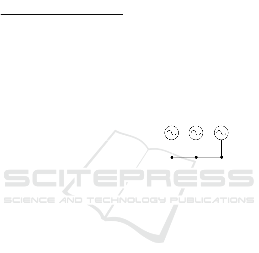
5.1 Six-node Network

This six-node three-phase network is a modiﬁca-

tion from the unbalanced network from (Sanseverino

et al., 2015), which is depicted by Fig. 2. There are

six nodes with three distributed generators and ﬁve li-

nes, which lead to three nonlinear equality constraint

in (6b). The size of the Hermitian symmetric ma-

trix variable W is 18 × 18. The coefﬁcients of the

power cost are set by c

= 0, c

= 4 and c

= 10

for each node and phase, respectively. The minimum

and maximum capacity of service voltage are set by

min

= 0.95pu, V

min

= 1.05pu for all nodes. The ini-

tial iteration of Algorithm 1 found rank(W

(0)

) = 8

with power cost 1086 ($/h), which is only a lower

bound of TOPF (14). SDR thus can not lead to feasi-

ble point for the original TOPF (6). After 5 iterations,

Algorithm 1 yields a rank-one solution with the po-

wer cost 1125 ($/h), with a 3.5% increase compared

to the lower bound 1086 ($/h).

DG1 DG2 DG3

Figure 2: Topology of the 6-node three-phase network.

5.2 Ten-node Network

This ten-node three-phase network is a modiﬁ-

cation of the unbalanced network modiﬁed from

(Dall’Anese et al., 2013), which is depicted by Fig.

3. There are ten nodes with two distributed generators

and nine lines, which lead to eight nonlinear equality

constraint in (6b). The size of the Hermitian symme-

tric matrix variable W is 30 × 30. The coefﬁcients of

the power cost are set by c

= 0, c

= 6 and c

= 30

for each node and phase, respectively. The minimum

and maximum capacity of service voltage are set by

min

= 0.95pu, V

min

= 1.05pu for all nodes. The ini-

tial iteration of Algorithm 1 found rank(W

(0)

) = 12

with power cost 1573 ($/h), which is only a lower

bound of TOPF (14). Again SDR can not ﬁnd even

a feasible point for original TOPF (6). After ten itera-

tions, the nonsmooth optimization Algorithm 1 yields

a rank-one matrix solution with the power cost 1652

($/h), which is a 5.0% increase compared to the lower

bound 1573 ($/h).

Three-phase Optimal Power Flow for Smart Grids by Iterative Nonsmooth Optimization

327

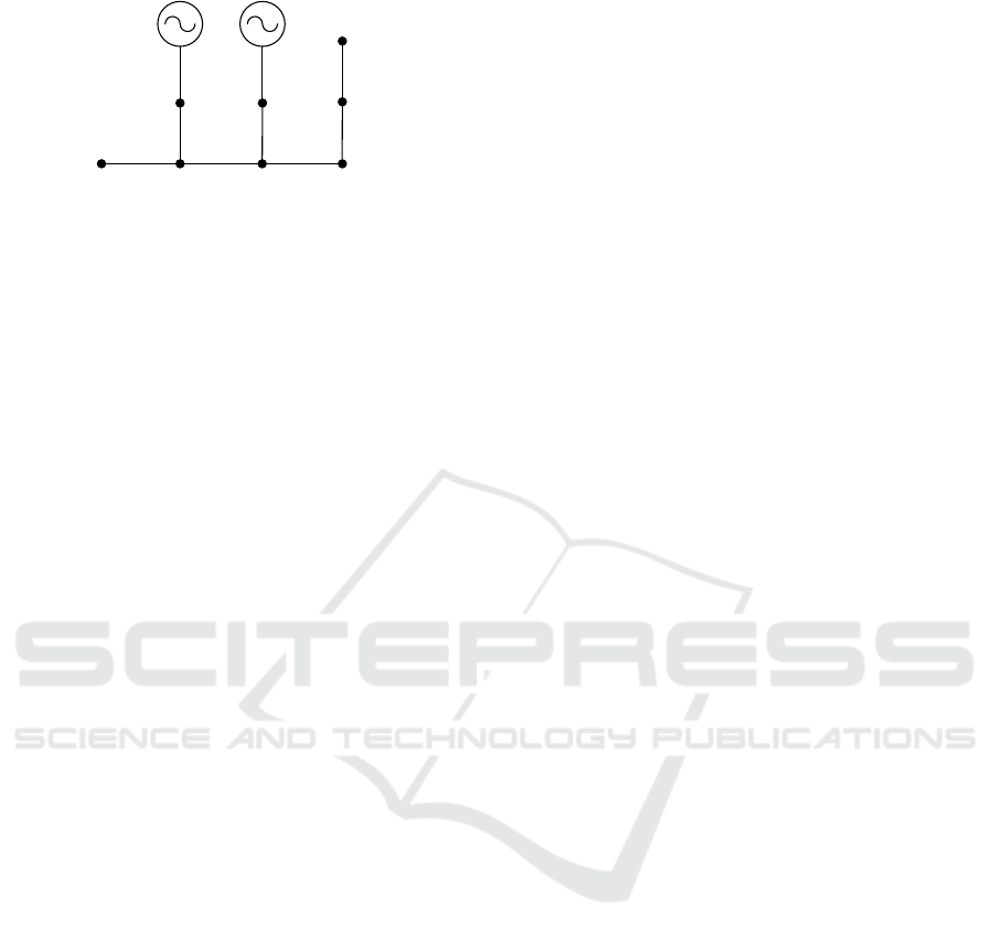
DG5 DG7

Figure 3: Topology of the 10-node three-phase network.

6 CONCLUSIONS

TOPF is a very computationally difﬁcult problem as

it involves multiple quadratic equality and indeﬁnite

quadratic inequality constraints of the bus intercon-

nections, hardware operating capacity and balance be-

tween power demand and supply. We have proposed

an iterative nonsmooth algorithm for its computatio-

nal solution. The provided simulations demonstrate

its merit. Its applications to larger scale TOPFs are

currently under consideration.

REFERENCES

Abdelaziz, M. M. A., Farag, H. E., El-Saadany, E. F., and

Mohamed, Y. A. R. I. (2013). A novel and genera-

lized three-phase power ﬂow algorithm for islanded

microgrids using a Newton trust region method. IEEE

Trans. Power Systems, 28(1):190–201.

Bukhsh, W., Grothey, A., McKinnon, K., and Trodden, P.

(2013). Local solutions of the optimal power ﬂow pro-

blem. IEEE Trans. Power Systems, 28(4):4780–4788.

Dall’Anese, E., Zhu, H., and Giannakis, G. B. (2013).

Distributed optimal power ﬂow for smart microgrids.

IEEE Trans. Smart Grid, 4(3):1464–1475.

Deshmukh, S., Natarajan, B., and Pahwa, A. (2012).

Voltage/var control in distribution networks via re-

active power injection through distributed generators.

IEEE Trans. Smart Grid, 3(3):1226–1234.

Farhangi, H. (2010). The path of the smart grid. IEEE

Power and Energy Magazine, 8:18–28.

Grant, M. and Boyd, S. (2014). CVX: Matlab soft-

ware for disciplined convex programming, version

2.1. http://cvxr.com/cvx.

Kersting, W. H. (2007). Distribution System Modeling and

Analysis. Boca Raton, FL, USA: CRC, 2rd edition.

Lavaei, J. and Low, S. H. (2012). Zero duality gap in opti-

mal power ﬂow problem. IEEE Trans. Power Systems,

27(1):92–107.

Madani, R., Sojoudi, S., and Lavaei, J. (2015). Convex re-

laxation for optimal power ﬂow problem: Mesh net-

works. IEEE Trans. Power Systems, 30:199–211.

Phan, H. A., Tuan, H. D., Kha, H. H., and Ngo, D. T. (2012).

Nonsmooth optimization for efﬁcient beamforming in

cognitive radio multicast transmission. IEEE Trans.

Signal Processing, 60(6):2941–2951.

Sanseverino, E. R., Quang, N. N., Di Silvestre, M. L., Guer-

rero, J. M., and Li, C. (2015). Optimal power ﬂow in

three-phase islanded microgrids with inverter interfa-

ced units. Electric Power Systems Research, 123:48–

56.

Shi, Y., Tuan, H. D., and Su, S. (2015). Nonsmooth opti-

mization for optimal power ﬂow. In Proc. of the 3rd

IEEE Global Conference on Signal and Information

Processing, pages 1–4.

Sturm, J. F. (1999). Using SeDuMi 1.02: A Matlab tool-

box for optimization over symmetric cones. Optim.

Methods Software, 11-12:625–653.

Tuan, H. D., Apkarian, P., Hosoe, S., and Tuy, H. (2000).

D.c. optimization approach to robust controls: the fe-

asibility problems. Inter. J. of Control, 73:89–104.

Yang, F. and Li, Z. (2016). Effects of balanced and un-

balanced distribution system modeling on power ﬂow

analysis. In Proc. of 2016 IEEE Power Energy So-

ciety Innovative Smart Grid Technologies Conference

(ISGT), pages 1–5.

Zimmerman, R. D., Murillo-Sanchez, C. E., and Thomas,

R. J. (2011). Matpower: Steady-state operations,

planning, and analysis tools for power systems re-

search and education. IEEE Trans. Power Systems,,

26(1):12–19.

SMARTGREENS 2017 - 6th International Conference on Smart Cities and Green ICT Systems

328