
Taming the Evolution of Big Data and its Technologies in BigGIS
A Conceptual Architectural Framework for Spatio-Temporal Analytics at Scale
Patrick Wiener
1
, Viliam Simko
2
and Jens Nimis
1
1
Karlsruhe University of Applied Sciences, Karlsruhe, Germany
2
FZI Research Center for Information Technology, Karlsruhe, Germany
Keywords:
Big Data, Geographic Information Systems, Software Architectures, Software Design Patterns, Data Pipelines.
Abstract:
In the era of spatio-temporal big data, geographic information systems have to deal with a myriad of big data
induced challenges such as scalability, flexibility or fault-tolerance. Furthermore, the rapid evolution of the
underlying, occasionally competing big data ecosystems inevitably needs to be taken into account from the
early system design phase. In order to generate valuable knowledge from spatio-temporal big data, a holistic
approach manifested in an appropriate architectural design is necessary, which is a non-trivial task with regards
to the tremendous design space. Therefore, we present the conceptual architectural framework of BigGIS, a
predictive and prescriptive spatio-temporal analytics platform, that integrates big data analytics, semantic web
technologies and visual analytics methodologies in our continuous refinement model.
1 INTRODUCTION
Geographic information systems (GIS) have long been
used to support humans in complex decision-making
processes (Crossland et al., 1995) such as transport
logistics, environment protection or civil planning.
They are supported by an ever-growing variety and
volume of new data sources such as hyperspectral im-
agery from unmanned aerial vehicles, real-time sensor
data streams, or open geodata initiatives and are often
expected to deliver their analysis results in a timely
or even interactive fashion (OGC, 2013). As the de-
scribed properties are the defining cornerstones in the
field of big data, it is inevitable that the respective
methodologies and technologies become integral part
of future GIS (Peng and Liangcun, 2014). Such big
data enabled GIS have to provide core functionalities
for spatio-temporal analytics with all the required sub-
tasks such as an integrated treatment of raster and vec-
tor data. Moreover, as big data itself provides a rapidly
developing ecosystems of tools and infrastructures, fu-
ture GIS will need to cope with heterogeneity not only
on data and use case but also on infrastructure level.
The manifold roles of humans in GIS decision-making
processes as users, experts and sometimes even as data
providers, have to be reflected in GIS by providing
appropriate interaction capabilities and resilience to
uncertainty. An application that fulfills all these differ-
ent and complex requirements may need to perform
a variety of tasks on the information that it processes.
A straightforward but inflexible approach to imple-
menting such applications would be to perform this
processing in one monolithic module. However, this
approach is likely to reduce the opportunities for refac-
toring code, optimizing it, or reusing it if similar pro-
cessing
(sub-)tasks
are required elsewhere within the
application or in other scenarios. Thus, decomposing
complex processing tasks into a series of discrete and
reusable components is a central idea of our BigGIS
conceptual architectural framework. The utilization of
the established pipes and filters pattern (Buschmann
et al., 2007) to construct the overall application can
improve performance, eases scalability and reusabil-
ity by allowing components that perform processing
and analysis tasks to be deployed and scaled indepen-
dently.
In summary, in this paper we pursue the goal to
provide a highly-flexible, modular, scalable and fault-
tolerant architectural framework for a wide range of
batch and streaming workloads to process and ana-
lyze heterogeneous and uncertain spatio-temporal data
at scale by leveraging existing big data technologies.
Thereby, we instantiate the continuous refinement
model of our BigGIS vision (Wiener et al., 2016).
To achieve the above goal, we first discuss related
work in Section 2. In Section 3, we describe four ex-
emplary BigGIS applications and therefrom derive the
architectural framework’s requirements. Section 4 is
90
Wiener, P., Simko, V. and Nimis, J.
Taming the Evolution of Big Data and its Technologies in BigGIS - A Conceptual Architectural Framework for Spatio-Temporal Analytics at Scale.
DOI: 10.5220/0006334200900101
In Proceedings of the 3rd International Conference on Geographical Information Systems Theory, Applications and Management (GISTAM 2017), pages 90-101
ISBN: 978-989-758-252-3
Copyright © 2017 by SCITEPRESS – Science and Technology Publications, Lda. All rights reserved

Domain Expert
Knowledge!
User!
Veracity (Uncertainty)!
Value (Knowledge)!
Smart Semantic Web
Services!
Indirect Expert Support!
Indirect Semantic Support!
Action!
Finding!
Direct Semantic !
Support!
Direct Expert!
Support!
System!
Human!
Data!
Visualization!
Model!
Remote
Sensing!
VGI!
Sensors!
...!
Archive!
Sources!
Continuous Refinement!
Figure 1: Continuous refinement model in BigGIS (Wiener
et al., 2016).
dedicated to the architectural elements of the frame-
work while Section 5 describes how they work together
along a user’s system interaction stages. To discuss
and illustrate our approach we show an example im-
plementation for one of the use cases in Section 6. We
conclude the paper and give an outlook on future work
in the last section.
2 RELATED WORK
In our previous work, we have introduced the vision of
BigGIS, a next generation geographic information sys-
tems shown in Figure 1 that allows for predictive and
prescriptive spatio-temporal analytics of geographic
big data (Wiener et al., 2016). We consider uncertainty
to be reciprocally related to generating new insights
and consequently knowledge. Thus, modeling uncer-
tainty is a crucial task. On an abstract level, our ap-
proach extends the knowledge generation model for
visual analytics (Sacha et al., 2014) in an integrated an-
alytics pipeline which blends big data analytics and se-
mantic web technologies on system-side with domain
expert knowledge on human-side, thereby allowing
expert and semantic knowledge to enter the pipeline at
arbitrary stages what we refer to as refinement gates.
By leveraging the continuous refinement model, we
present a holistic approach that explicitly deals with
all big data dimensions. By integrating the user in the
process, computers can learn from the cognitive and
perceptive skills of human analysis to create hidden
connections between data and the problem domain.
This helps to decrease the noise and uncertainty and
allows to build up trust in the analysis results on user
side which will eventually lead to an increasing likeli-
hood of relevant findings and generated knowledge.
The conversion of our vision into a more concrete
architectural framework is at its heart a system design
issue and as such should benefit from and rely on the
extensive experience in this field which is externalized
in general software architecture patterns (Buschmann
et al., 2007). E.g. layering and pipes and filters are
two often occurring and re-used architecture patterns
where the latter also is the foundation of the BigGIS ar-
chitecture framework. The BigGIS framework design
decision to build up on the pipes and filters pattern
is in line with prominent representatives of general
big data architecture such as the lambda architecture
(Marz and Warren, 2013) or kappa architecture (Kreps,
2014). They both are based on the pipes and filters
pattern while trying to cope with the tension between
batch and stream processing in big data analytics.
There exists a number of big data systems and
platforms that follow a pipes and filters related ap-
proach. StreamPipes (Riemer et al., 2015) provides
a user-oriented interface for managing complex event
processing on top of big data streams. It leverages
semantic web technologies to describe elements of
the pipelines which are then running on a variety of
distributed big data platforms. Reliable and scalable
messaging across the various components and tech-
nologies is achieved through Apache Kafka
1
. The
KNIME Analytics Platform (Berthold et al., 2007) pro-
vides a GUI for building data processing pipelines that
can run locally or in a KNIME cluster. A so-called
KNIME workflow is composed of nodes connected
by edges between their input/output ports. When exe-
cuted, pipelines operate in batch manner, exchanging
data tables, predictive models, parameters or connec-
tions to external services. The KNIME platform pro-
vides generic as well as domain-specific nodes for, e.g.,
chromosome analysis, machine learning, time series
analytics. The purpose of Apache NiFi (Apache Foun-
dation, 2016) is to allow for high-performance data
flow management throughout an enterprise. Therefore,
it provides a user-oriented graphical interface utilizing
powerful and scalable directed graphs to capture data
routing, transformation and system mediation logic.
However, at the time of writing, these platforms do
not provide spatial analytics capabilities for the wide
spectrum of GIS use cases in order to address all big
data induced requirements.
Even more specific within the spatio-temporal ana-
lytics domain a number of systems and libraries have
originated, e.g. PlanetSense (Thakur et al., 2015),
ArcGIS Big Data Analytics (Esri, 2016), GeoTrel-
lis (Eclipse Foundation, 2016), and many more. While
they all provide certain functionality within the scope
of BigGIS’ applications, with their respective align-
ment they only address a subset of the use cases and
derived requirements presented in the following.
1
https://kafka.apache.org/
Taming the Evolution of Big Data and its Technologies in BigGIS - A Conceptual Architectural Framework for Spatio-Temporal Analytics
at Scale
91

3 MOTIVATING USE CASES
In this section, we present four motivating use cases
which demonstrate different aspects of geospatial and
spatio-temporal analytics that we want to support in
BigGIS in a scalable way using the state-of-the-art
technologies from the big data domain. An overview
of all use cases is summarized in Table 1 and the re-
sulting requirements are discussed in Subsection 3.5.
3.1 Hot Spot Analysis on New York Taxi
Drop-offs
This use case is motivated by the ACM SIGSPATIAL
GISCUP 2016 competition which aims at finding the
top 50 hot spots in space and time in terms of taxi
drop-off locations and passenger counts by comput-
ing the Getis-Ord G
∗
statistics (Ord and Getis, 1995).
The dataset contains taxi drop-offs from New York,
years 2009-2015. Computing the G
∗
statistics in a grid
involves aggregation of points into grid cells, comput-
ing the convolution, sorting and optionally computing
the mean and standard deviation of the whole dataset.
A graphical overview of the pipeline is depicted in
Figure 2.
Select Extent
and Time Interval
Read / Stream
the data
Aggregate to grid
Convolve
Aggregate to grid
Top 50 cells Show on map
Figure 2: Hot spot analysis pipeline based on Getis-Ord G
∗
statistics.
Files are stored in HDFS
2
(Hadoop Distributed File
System) using CSV (comma separated values) format;
2GB per month of data. Every row represents a single
taxi drop-off whereas the columns show corresponding
features such as latitude, longitude, time and passen-
ger count. The data points have to be aggregated into
a spatio-temporal grid with a granularity of approx.
100 m × 100 m × 1 day
. The grid cells are then con-
voluted with their neighbour cells (queen-distance of
one cell, i.e., 27 cells in a space-time cube) and the top
50 cells are then selected.
If the actual z-scores need to be computed, the grid-
based G
∗
algorithm is used (Def. 1) which requires the
mean and standard deviation of the whole dataset.
2
http://hadoop.apache.org/
Def. 1
(
G
∗
in a grid)
.
Assuming a notation
X
op
◦W
to denote a focal operation
op
applied on an n-
dimensional grid
X
with a focal window determined
by an n-dimensional matrix
W
. The function
G
∗
can
be expressed as follows:
G
∗
(X,W,N,M,S) =
X
sum
◦ W − M.
∑
w∈W
w
S
q
N.
∑
w∈W
w
2
−(
∑
w∈W
w)
2
N−1
where:
• X is the input grid.
• W is a weight matrix of values between 0 and 1.
• N represents the number of all cells in X.
• M represents the global mean of X.
• S represents the global standard deviation of X.
In the competition, Apache Spark
3
is used for com-
puting the space-time cubes of the datasets restricted
to year 2015 and to an envelope encompassing the five
New York City boroughs.
This is a typical batch processing use case which
can be extended to a stream processing application,
e.g, by updating the top 50 hot spots on-the-fly. There
are multiple parameters that can be configured by the
users including cell size, the number of top-k hot spots
returned or the spatio-temporal extent of the analysis.
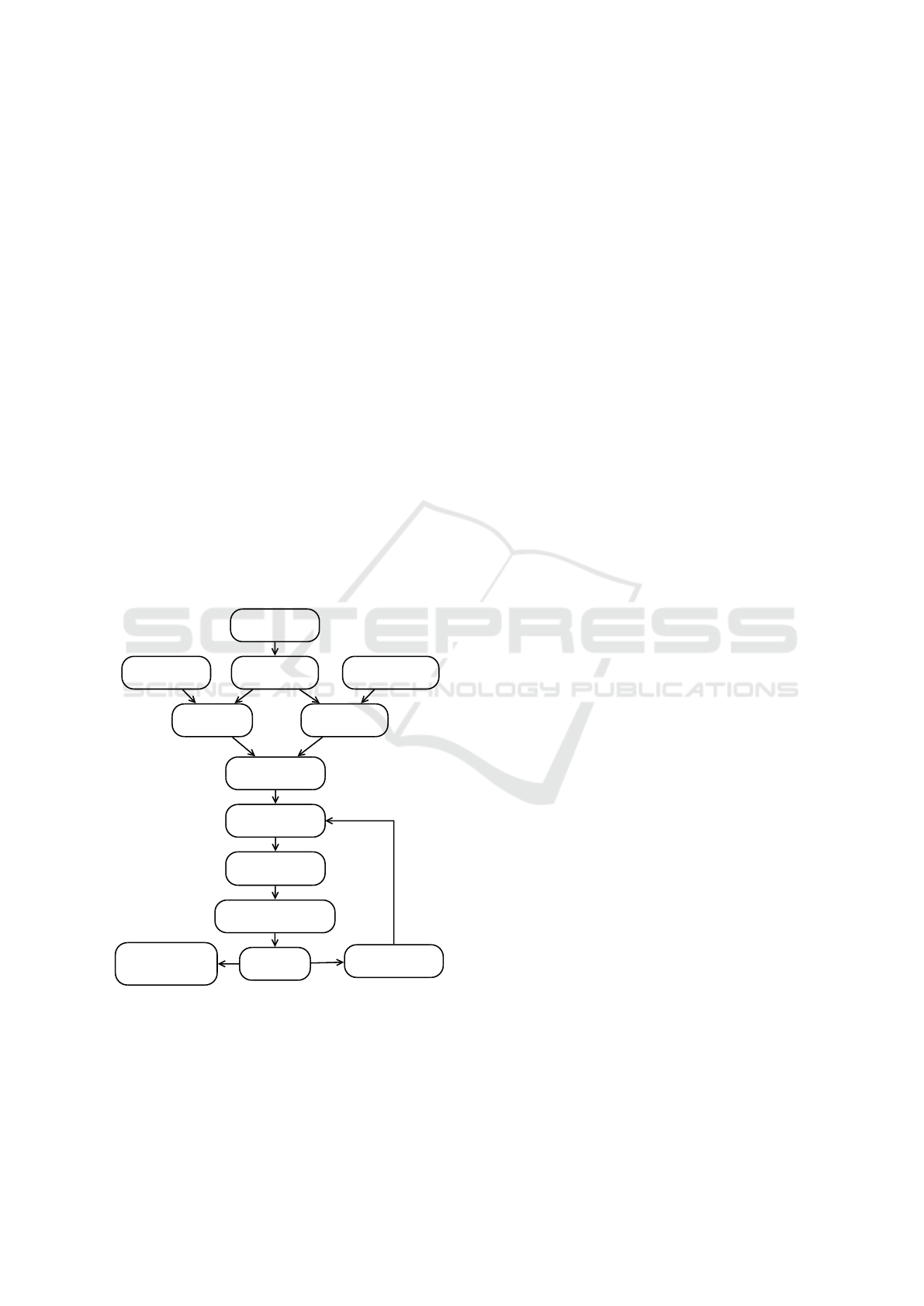
3.2 Computing NDVI/NDWI from
Landsat Images
This is a raster processing use case that involves lo-
cal map algebra operations (Tomlin, 1990) applied on
a multiband raster. We use the GeoTrellis (Eclipse
Foundation, 2016) library for distributed raster pro-
cesssing which splits an input raster into uniform tiles
indexed using a space filling curve. The use case
is loosely inspired by the GeoTrellis landsat tutorial
project (Emanuele, 2016). It involves the following
steps: (1) Discovery of landsat images. (2) Down-
loading the discovered GeoTIFF rasters from Amazon
S3 cloud. (3) Creating a 3-band GeoTIFF from the
red, green and nir (near infrared) bands masked with
the quality assessment (QA) band. (4) Computing
normalized differenced vegetation index (NDVI) and
normalized difference water index (NDWI) from the
red, green and near infrared bands. (5) Reprojecting
the GeoTIFF into WGS-84
4
projection (6) Tiling and
indexing of the raster into a GeoTrellis catalog (using
a space-filling curve) (7) Building a tile pyramid for
different zoom levels that can be served to web clients
in an efficient manner given
x/y/z
coordinates. An
overview of the pipeline is shown in Figure 3.
3
https://spark.apache.org/
4
WGS 84 / Pseudo-Mercator, http://epsg.io/3857
GISTAM 2017 - 3rd International Conference on Geographical Information Systems Theory, Applications and Management
92
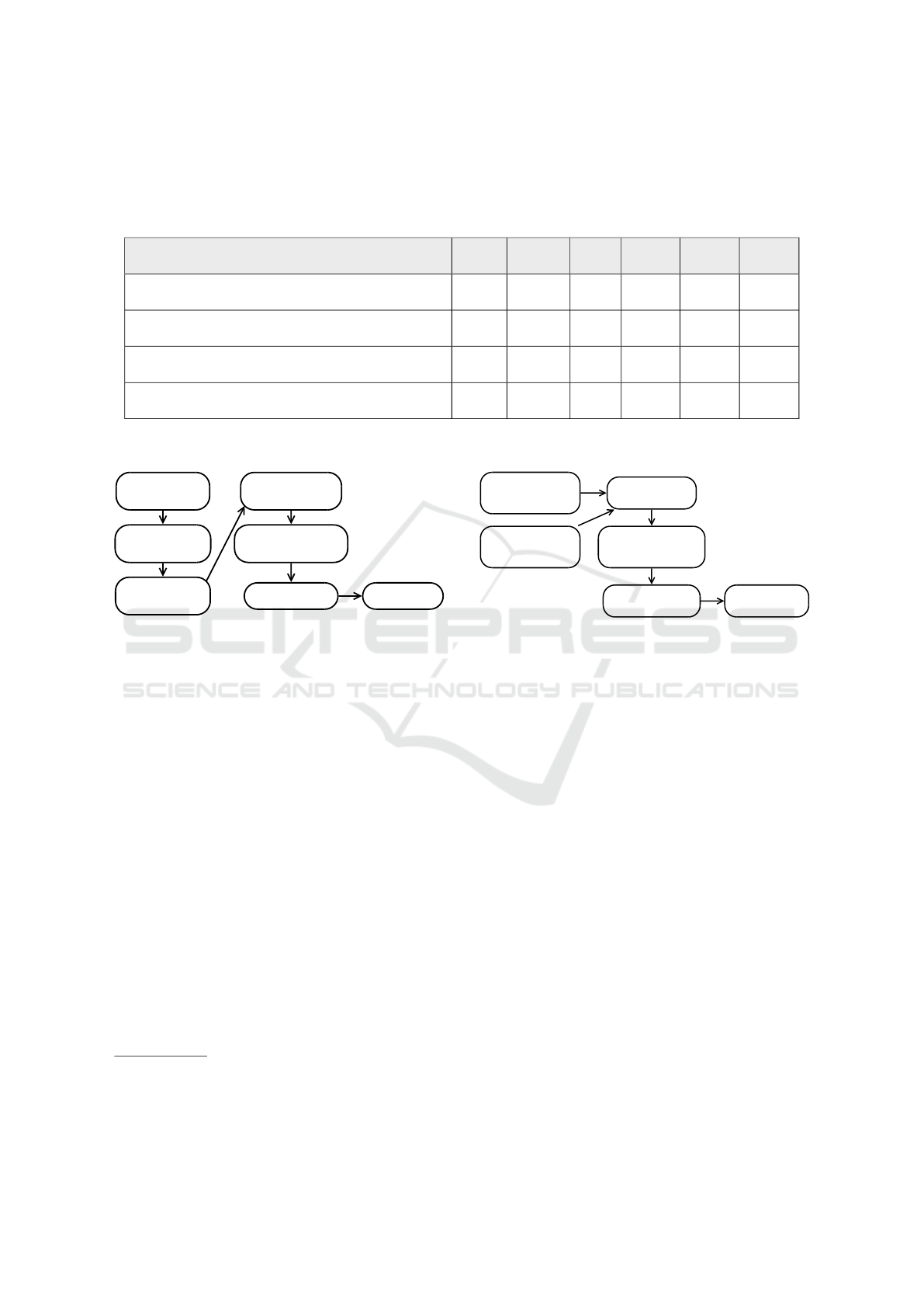
Table 1: Summary of use cases presented as a motivation.
Batch
processing: Data processed once on request till the end of
the dataset; Stream processing: Data continously processed from a potentially infinite stream; Time dimension: The data are
located in space and time.
Raster
processing: Usually GeoTIFFs, including map algebra operations;
Vector
processing: Usually
point measurements;
Model
: Uses some prediciton model such as SVM, Logistic regression, etc. Involves training, prediction
and evaluation of the model.
Batch Stream Time Raster Vector Model
Hot Spot Analysis on New York Taxi Drop-offs X (X) X × X ×
Computing NDVI/NDWI from Landsat Images X (X) × X × ×
Stream Enrichment × X X X X ×
Land Use Classification & Change Detection X X X X X X
Legend: X Yes, × No, (X) Can be extended
Discover landsat
images
Download geotiffs
from Amazon
Show on map
Store into
geotrellis catalog
Mask with QA band
(local op)
Compute NDVI+NDWI
(local op)
Build pyramid
Figure 3: NDVI/NDWI computation pipeline for Landsat
images.
3.3 Stream Enrichment
An overview of this scenario is depicted in Figure 4.
The goal is to treat historical and newly measured
temperatures from weather stations
5
as a stream of
input vectors (Def. 2) that has to be enriched with
additional information from raster and vector layers –
output vectors (Def. 3). Besides the air temperatures,
the stream may contain additional features, such as
humidity or wind speed/direction.
Def. 2
(Input vector)
.
A single measurement from
weather station id is encoded as a vector:
IN
n
= (id,ts,lat, lon,temp, hum,. .. ,wind)
• ts is the timestamp of the measurement
• lat,lon are geographical coordinates in WGS-84
• temp,hum, .. .,wind
are measured values such as
air temperature, humidity, wind speed etc.
Envisat rasters represent hourly LST (Land Surface
Temperature) readings with pixels of size
0.05 ×
5
For evaluation purposes, we use weather stations from
Deutscher Wetterdienst, LUBW Landesanstalt f
¨
ur Umwelt,
Messungen und Naturschutz Baden-W
¨
urttemberg and our
own LoRA-based sensors.
Receive measurement
from a weather station
(input vector)
Find neighbour
ENVISAT pixels
Find intersection with
ATKIS polygons
(area per land use class)
Pick top 3 classes
Generate enriched
output vector
Pull measurements
from a weather station
(input vector)
Figure 4: Overview of the stream enrichment pipeline.
0.05 deg
(i.e.
5.6 × 3.7 km
in Baden-W
¨
urttemberg).
In the analysis, the nearest pixels were needed for the
analysis. Although the satellites provide hourly scans
of the same region, gaps might have occurred due to
bad weather conditions or other factors, resulting in
NA values. The vector layer is the LUBW ATKIS
database that contains land use classification polygons
for regions such as forest, urban area, railway etc.
Def. 3
(Enriched output vector)
.
For a single mea-
surement
IN
n
= (id,ts,lat, lon,temp,hum,.. ., wind)
as defined in Def. 2, we construct an output vector
OUT
n
as follows:
OUT
n
= (id,ts, lat,lon,temp,hum, ...,wind,
pdist
1
,lst
1
,c
#1
1
,a
#1
1
,c
#2
1
,a
#2
1
,c
#3
1
,a
#3
1
,
.. .,
pdist
9
,lst
9
,c
#1
9
,a
#1
9
,c
#2
9
,a
#2
9
,c
#3
9
,a
#3
9
)
There are potentially nine raster pixels
i ∈ {1,.. ., 9}
that are nearest to the location
(ts,lat,lon)
. For a
given pixel
i
, let
lst
i
be its land surface temperature
and
pdist
i
be the distance from the pixel center to the
location
(lat,lon)
. Let
c
# j
i
be the land use class of
the ATKIS polygon that has the
j
-th largest area of
intersection a
# j
i
with the pixel i.
The stream of output vectors is passed through a
Taming the Evolution of Big Data and its Technologies in BigGIS - A Conceptual Architectural Framework for Spatio-Temporal Analytics
at Scale
93
dedicated queue, e.g. in Apache Kafka, and can be
further processed in a distributed manner.
3.4 Land Use Classification and Change
Detection
This scenario involves distributed raster processing
combined with machine learning. The goal is to auto-
matically detect changes in the land use classification
based on aerial/satellite imagery. The challenge here is
that land use classes, indicating how people are using
the land, have a higher semantic meaning and thus
cannot be directly determined from the images. On the
other hand, land cover classes, indicating the physical
land type (e.g. green area, water etc.), can be deter-
mined by analyzing the images in an automated way.
Land use classification databases are updated manually
by domain experts based on land cover surveys from
multiple years with the help of predefined compatibil-
ity criteria between land use and land cover classes
(e.g. how much coverage of class A may be contained
in a land use class B). Some of these criteria can be
checked automatically thus minimizing the amount of
work for domain experts. An overview of the whole
use case is depicted in Figure 5.
Check compatibility criteria
(land use vs. land cover)
User chooses initial
training area
User chooses
area for classification
Evaluation / Feedback
from users (pixels)
Raster ingest
Tiling and indexing
using SFC
Query tiles
for initial training
Tiles to Pixels
Present results
to the user
Pixels to Tiles
on-line
prediction / training
Query tiles
for classification
Update land use
classification database
(manually)
Figure 5: Land use classification and change detection
pipeline.
Land use classification is encoded as polygons with
an attached class. The aerial and satellite images are
encoded as multiband rasters. In order to support dis-
tributed processing, polygons have to be indexed using
a space-filling curve (SFC). The rasters have to be
cut into uniform tiles (e.g.
256 × 256 px
), organized
in a grid and also indexed using a SFC for efficient
distributed processing. An important architectural fea-
ture, besides the local and focal map algebra operations
(Tomlin, 1990), is the ability to convert raster tiles into
a stream of individual pixels (Def. 4).
Def. 4
(Converting Tiles to a Stream of Pixels)
.
Let
T
be a square multiband tile with n + 1 bands.
T = (T
idx
,T
v
1
,. .. ,T
v
n
)
T
idx
is a composed index containing the SFC index of
the tile and row/column pixel coordinates within the
tile.
T
v
1
,. .. ,T
v
n
represent the pixel values, (e.g. red,
green, blue, nir). Then, we define a mapping function
from tile to pixels as follows:
ψ : T 7→ {T
i, j
: ∀i, j}
Notice that result of
ψ(T )
is a sample set, where each
element is a tuple (idx, v
1
,. .. ,v
n
).
We can also define a corresponding inverse func-
tion
ψ
−1
that converts stream of pixels back to a multi-
band raster.
The pixelization function
ψ
preprocesses the raster
tiles into a form suitable for pixel classification. Here,
we can either follow the traditional approach or the on-
line stream learning approach. In the former case, the
dataset is split into training and testing set (manually
or automatically). The training set is used for building
the classification model whose prediction performance
is crossvalidated on the testing set. In the latter, the
prediction performance of a model is continuously
evaluated and adjusted (if supported by the model)
or retrained after reaching a certain error threshold.
In both cases, the classifier converts incoming pixels
into a new stream of predictions. These are converted
back to raster tiles using the aforementioned inverse
function ψ
−1
.
After the classification phase, the compatibility cri-
teria between the land use classes and newly predicted
land cover classes can be checked and presented to the
domain expert for manual inspection. Feedback from
the user can be treated as a source of training samples
to improve classification accuracy forming a feedback
loop.
3.5 Requirements
As the aforementioned use cases demonstrate, the
range of application is manifold. Thus, defining dis-
tinct functional and non-functional requirements is not
feasible, which is why we refer to the more general
term of requirements in the following.
GISTAM 2017 - 3rd International Conference on Geographical Information Systems Theory, Applications and Management
94

3.5.1 Spatial and Temporal Analytics Support
Regarding the domain of spatio-temporal big data ana-
lytics, it is mandatory that a big data enabled GIS must
provide support for spatio-temporal analytics. For in-
stance, this can be map algebra operations on raster
data, vector/raster conversions, spatial time series anal-
ysis, or multilayer multiband capabilities.
3.5.2 Heterogeneity-Awareness
Considering the rapidly growing amount of data
sources especially in the space-time context, e.g. hy-
perspectral imagery from unmanned aerial vehicles,
it is necessary to provide means to (1) easily inte-
grate these heterogeneous data sources through de-
fined wrappers and transformations in a required and
more standardized format before analyses, as well as
(2) extend the pool of possible data sources to new
ones.
3.5.3 Uncertainty-Awareness
Since noise and erroneous data are natural in the real
world, additional provenance and metadata informa-
tion, e.g., the type and accuracy of a given sensor, can
be beneficial for modeling these inherent uncertainties
in data. Thus, the system should allow annotating the
semantic information and relation of data sources.
3.5.4 User Integration
While computers are good at data management and
processing, the humans’ cognitive and perceptive skills
allow to establish hidden connections between the
data and the problem domain. Thus, providing a set
of suitable web-based visualizations is obligatory, to
(1) present analyzed results to users in an adequate
manner, (2) allow expert users to visually explore the
results, (3) provide a channel to manipulate computa-
tion at arbitrary stages in the processing pipeline.
3.5.5 Technology-Agnosticism
The ever ongoing evolution in computer science in
terms of advancements in big data analytics, for in-
stance enhanced distributed machine learning algo-
rithms and newly arising open source big data frame-
works, introduce crucial requirements that dictate our
design approach. Choosing one technology in favor
of another can therefore cause strong limitations in
terms of applicability to a wider range of use cases,
thus introducing lock-in effects and inflexibility. As a
consequence, the architectural design should account
for these circumstances such that it is possible to lever-
age multiple underlying big data technologies for dis-
tributed batch, stream processing or machine learning
as needed. By splitting up computational monoliths
in a variety of discrete blocks, each serving a certain
functionality and potentially running on different big
data technology, invokes the requirement of having a
standardized and reliable way of communication as
well as repositories to store these artifacts for later use.
Therefore, intermediate results of these computational
blocks should be made available for arbitrary consec-
utive ones such that it is possible to apply different
functions on the same data in parallel.
4 ARCHITECTURAL ELEMENTS
Designing a conceptual architectural framework,
which accounts for the aforementioned requirements,
involves decomposing the design in various architec-
tural elements that are presented in the following.
Def. 5
(BigGIS)
.
The conceptual architectural frame-
work of
BigGIS
is formally described as a tuple
(P,S, R,A), where:
• P is a set of pipelines
• S is a set of services
• R is a set of repositories
• A is a set of user actions
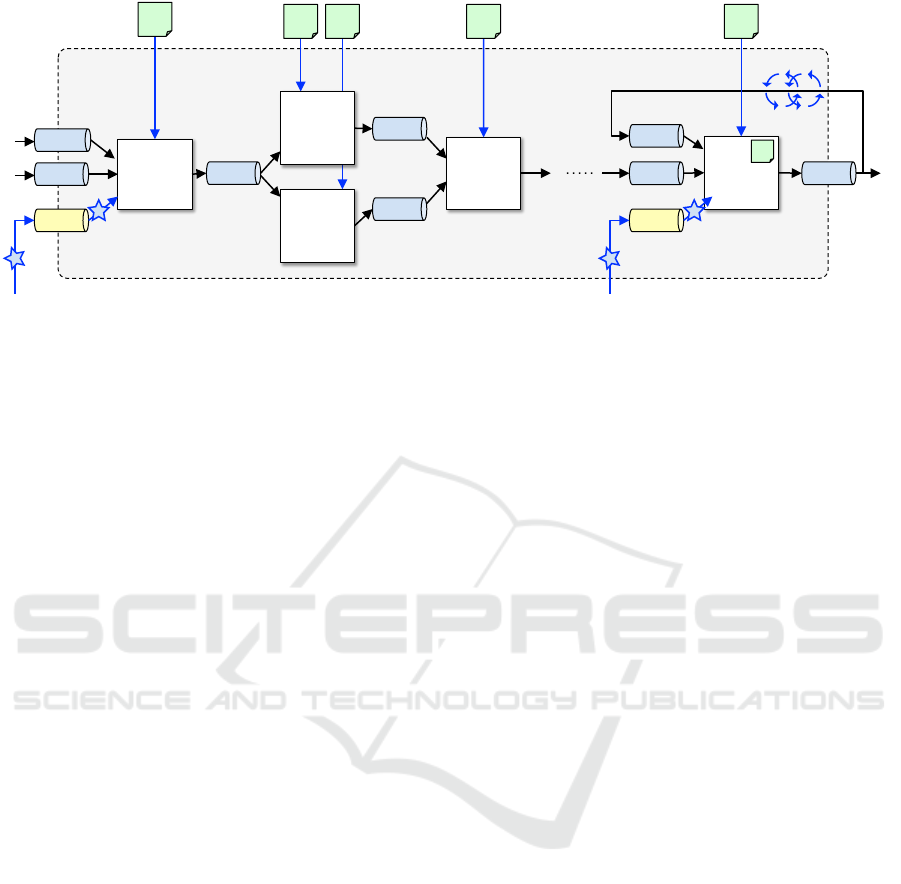
4.1 Pipelines
In BigGIS, functionalities are encapsulated in discrete
and reusable computational blocks called nodes each
of which follow the single responsibility principle and
perform only one specific task, e.g., download source
data, perform spatial binning, or apply a classifier to
predict the land use class. Multiple consecutive nodes
are interconnected through dedicated queues to trans-
fer data in a standardized and homogeneous format
between nodes. The resulting processing chain allows
for a combination of these nodes into a use case spe-
cific pipeline as is generically shown in Figure 6.
Def. 6
(Pipeline)
.
A pipeline
p
is formally described
as a tuple (N,Q), where:
• N is a set of nodes
• Q is a set of queues
4.1.1 Nodes
A node
n
is responsible for processing and analyzing
input data that it consumes from one or more input
queues Q
in
by subscribing to dedicated topics T . In-
Taming the Evolution of Big Data and its Technologies in BigGIS - A Conceptual Architectural Framework for Spatio-Temporal Analytics
at Scale
95
node 1
!
pipeline p
i!
node 4
!
node 3
!
node n
!
c
4!
c
n!
c
1!
c
2!
c
3!
node 2
!
m
!
Figure 6: A pipeline in BigGIS is composed of consecutive nodes and queues, in which each node
i
performs a dedicated
processing task, e.g. normalizing, cleansing, filtering, or analytical task, e.g. calculating statistics, applying pre-trained machine
learning models
m
, on the received input data (input queues). Generally, the results are propagated downstream (output queues)
for further processing but can also be back propagated for iterative algorithms. Configuration parameters
c
i
describe the setup a
node. Special input queues called refinement gates allow for external user knowledge to update/change the corresponding node
in the form of periodical refinement events (F).
side a node, task specific functions
F
are consecutively
applied whenever new data
D
is received on the input
side to further manipulate and refine the input data.
In addition, configuration parameters
c
from the con-
fig repository are used to configure and parametrize
the node. The results of the computation is then pub-
lished back to one or more output queues
Q
out
on new
topics
T
. By constraining the semantics of the input
data queue mechanism, we want to solve the follow-
ing issues: (1) preventing deadlocks, (2) maximizing
performance.
While it can be necessary for certain nodes to
join multiple input queues together, this simplification
avoids deadlocks and idling nodes which increases the
performance. Besides that, consecutive nodes need not
to be deployed on the same computational framework.
Thus, a node can run on the most suitable underlying
big data framework and in a distributed manner. To
continuously refine results nodes can subscribe to their
own output queue and consume the results
D
∗
, e.g. to
perform iterative computation. An essential property
of a node is its metadata
meta
which provides infor-
mation characterizing the node, for instance what the
node’s job is, or what type of input data and formats
it can handle. A special type of node is the machine
learning node where a suitable pre-trained machine
learning model
m
of set
M
is loaded inside the node
as shown in Figure 7, to perform predictive analysis,
e.g. to classify the land use class as a crucial part to
automated change detection as depicted in Section 3.4.
Def. 7.
(Node). A node
n
is formally described as a
tuple (Q
in
,Q
out
,F,c, meta,m), where:
• Q
in
is a set of input queues
• Q
out
is a set of output queues
• F is a set of functions
• c
are node specific configurations and parameters
• meta is the metadata description
• m
is a machine learning model of set M (optional)
4.1.2 Queues
A queue
q
is a communication channel either between
(1) external and internal components, e.g. from exter-
nal data sources and nodes, (2) two or more consecu-
tive nodes, (3) nodes and data sinks, e.g. a database
or visual analytics user interfaces. Queues are an inte-
gral part of BigGIS as they provide a flexible way to
decouple arbitrary components such as two or more
consecutive nodes. A queue carries data
d
associated
with a certain topic
t
that has been published by spe-
cific node. Arbitrary number of subsequent nodes can
then register for this topic in order to dequeue the data
in a first-in-first-out manner. Queues can either be
classified as input queues
Q
in
or as output queues
Q
out
with respect to a certain node. The data can be the
actual data, e.g., a stream of vector data from weather
stations, or metadata information, e.g., storage loca-
tion of raster images. Besides, there are special input
queues called refinement gates
Q
rgate
that contain pe-
riodical refinement events (
F
) representing external
user knowledge that will trigger a certain update in
the corresponding node, e.g. specifying the number
of top-k hot spots to be returned by a top-k hot spots
node, or providing new training data samples for a
machine learning node, as shown in Figure 7.
Def. 8.
(Queue). A queue
q
is formally described as a
tuple (T, D), where:
• T is a set of topics
• D is the available data
GISTAM 2017 - 3rd International Conference on Geographical Information Systems Theory, Applications and Management
96

node i!
q
i,rgate!
D
h!
D
*!
q
i,in2!
q
i,in1!
D
!
D
g!
D
f!
c
i!
f(D,D
*
, )
!
g(D
f
)
!
h(D
g
)
!
q
i,out1!
m
!
Figure 7: An iterative machine learning node
i
making pre-
dictions on data
D
from corresponding input queue
q
i,in
by
applying the functions
f ,g,h
and publishing the results on
the output queue
q
i,out
, while in this case the predicted output
D
∗
is self-subscribed. User knowledge, e.g. for parameter
tuning, gets injected through the refinement gate q
i,rgate
.
4.2 Services
Self-sustained units of functionalities for a given task
that expose a distinct interface for interaction are called
services
S
. In BigGIS, a service can be classified in
three categories that are (1) provider, (2) integrator,
(3) manager. Providers expose adapters to connect
to certain data sources and data sinks. Reasoning on
the semantic metadata as part of the data integration
process is the task of the integrators, which are re-
sponsible for data homogenization and normalization.
Managers take care of the deployment and supervision
of pipelines and nodes as well as handling user actions
such as updating configurations and parameters, or
injecting new refinement events to refinement gates.
Def. 9.
(Service). A service
s
is formally described as
a tuple (s
t
,s
n
), where:
• s
t
is the service type
• s
n
is the service name
4.2.1 Data Source Service
The data source service provides a set of adapters to
external data sources, e.g. satellite images stored in
Amazon S3 buckets, volunteered geographic informa-
tion and other open data initiatives through REST API
calls, or streaming sources such as sensor readings
from weather stations.
4.2.2 Data Sink Service
Like the aforementioned data source service, the data
sink service provides a set of adapters to expose the
processed and analyzed data from the last output
queues of a pipeline to a variety of different data sinks,
e.g., databases for persistent storage, REST APIs for
exposing the top-k hot spots, or visual representations
such as real-time monitoring dashboards or specific
visual analytic views. The latter presents a fundamen-
tal element in BigGIS that enables users to visually
explore the data and analyses results thereby allow-
ing them (1) to reason on and interpret the massive
amounts of spatio-temporal big data to gain insights
into causalities of determining factors for a given prob-
lem domain that would otherwise not be easily iden-
tified, as well as (2) to adjust specific parameters in
deployed nodes of pipelines.
4.2.3 Linked API Service
The linked API service is a semantic web service
that helps integrating various data sources (integrator),
which are typically exposing diverse data formats and
data schemas. In collaboration with the data source
service and the data source repository, it is possible to
perform a smart data integration by building on top of
exisiting and well-established ontologies, e.g. QUDT
6
,
or GeoSPARQL
7
in order to cope with heterogeneous
data sources. This allows for (1) traceability and prove-
nance information of spatio-temporal big data, (2) a
robust data integration, possibly even of open linked
geo data sources, (3) a flexible approach to cope with
the heterogeneity in data input and output formats.
4.2.4 Cognitive App Service
The cognitive app service enables pipeline and node
deployment as well as user action mediation between
visual analytics views, nodes and the underlying big
data frameworks (manager). When necessary, this
service updates configuration parameters of nodes in
the configuration repository and propagates refinement
events to update functions of dedicated nodes in the
pipeline through refinement gates input queues. In
addition, the cognitive app service is context-aware
which means that besides the actual deployment of
nodes and pipelines it further supervises the execution
of the nodes on the underlying big data frameworks.
4.3 Repositories
Dedicated stores for various components in BigGIS are
called repositories
R
. Repositories serve two specific
purposes (1) conduct metadata information such as
information about semantically described data sources,
e.g. resolution and update cycles of satellite imagery
or pipeline descriptions for performing complex ana-
lytical tasks, e.g. land use classification, (2) serve as a
storage location from which software artifacts such as
6
http://www.qudt.org/
7
http://www.opengeospatial.org/standards/geosparql
Taming the Evolution of Big Data and its Technologies in BigGIS - A Conceptual Architectural Framework for Spatio-Temporal Analytics
at Scale
97

packaged nodes or visualizations may be retrieved and
deployed on the underlying big data infrastructure.
Def. 10.
(Repository). A repository
r
is formally
described as a tuple (r
t
,r
n
), where:
• r
t
is the repository type, either metadata or artifact
storage
• r
n
is the repository name
4.3.1 Data Source Repository
The data source repository contains semantically anno-
tated descriptions of various data sources that model
complex correlations in a graphical approach based on
RDF
8
(resource description framework).
4.3.2 Model Repository
The model repository stores pre-trained machine learn-
ing models in a reusable way, e.g., PMML (Guazzelli
et al., 2009), so that they can be loaded inside a dedi-
cated machine learning node for performing predictive
analyses on new data.
4.3.3 Configuration Repository
The configuration repository contains relevant config-
uration files and parameters for running nodes.
4.3.4 Pipeline Repository
The pipeline repository stores templates and descrip-
tions for performing recurrent and complex analytical
tasks. A description contains various useful informa-
tion, e.g. what data sources and nodes are used, how
they are plugged together, or what the parameter val-
ues are in order to get a satisfactory prediction quality.
This can be used as a good starting point for non-expert
users as well as for expert users who can focus on the
interpretation and reasoning rather than building a cer-
tain pipeline over and over again.
4.3.5 Node Repository
The node repository is an artifact store that comprises
all nodes. The artifact itself contains the pre-packaged
source code and necessary libraries to perform the task
as well as a metadata description of the node, e.g.,
what the node’s task is, what type of input data it can
handle, what type of output data it produces, or what
underlying big data framework it utilizes.
8
https://www.w3.org/RDF/
4.3.6 Visualization Repository
The visualization repository is another artifact store
that contains predefined web-based graphical user in-
terfaces. On one hand, this could be a configurable
real-time dashboard to monitor the analysis results. On
the other hand, this could be interactive visual analyt-
ics views that enable users to interact with dedicated
nodes inside pipelines while visually exploring the
data, e.g., changing the time window for computing
the mean over the resulting finite set of data elements
or adjusting parameters in a machine learning node.
4.4 User Actions
User actions
A
are a crucial part of BigGIS since they
enable the user to interact with the system. Gener-
ally, there are various types of actions possible. Thus,
we differentiate between (1) non-interactive user ac-
tions, e.g., selecting relevant data sources or defining
pipelines of nodes, and (2) interactive user actions
that are characterized by visualizations to support the
knowledge generation on user side. The latter gives
the user the opportunity to visually explore the results,
reason on them and trigger adequate changes accord-
ing to the level of domain knowledge. User actions on
visualization elements, e.g., moving a slider to change
top-k hot spots or calculating spatio-temporal statistics
for a given spatial extent, generate tangible, unique
responses from a visual analytics system (Sacha et al.,
2014) such as BigGIS. By applying adjustments on the
visual analytics views the user implicitly manipulates
the affected processing nodes
N
at predefined stages
of a given pipeline by injecting refinement events over
a set of topics
T
rgate
for refinement gate input queues.
Thus, enhancing the creativity and curiosity of the user
during the course of exploration. From now on, we
refer to user actions as interactive user actions.
Def. 11.
(User Action). A user action
a
is formally
described as a tuple (a
t
,N,T
rgate
,c), where:
• a
t
is user action type
• N is a set of nodes that are affected by changes
• T
rgate
is a set of topics for refinement gate queues
• c
are node specific configurations and parameters
5 CONCEPTUAL
ARCHITECTURAL
FRAMEWORK OF BigGIS
This section introduces the conceptual architectural
framework of BigGIS and how the previously pre-
GISTAM 2017 - 3rd International Conference on Geographical Information Systems Theory, Applications and Management
98
o
1!
node 1
!
c
i!
node n
!
pipeline p
i!
Linked
API!
Cognitive
App!
Pipeline!
Repository!
q
1,rgate!
Data Source!
Repository!
Data
Source(s)!
Remote
Sensing!
VGI!
Sensors!
...!
Archive!
Visualization!
Repository!
Model!
Repository!
User!
Action!
Finding!
Human!Sources!
System!
Visual
Analytics!
RT-
Monitor!
...!
q
1,in2!
q
n,out2!
q
1,in1!
q
n,out1!
D
!
Node!
Repository!
Data
Sink(s)!
Data
Storages!
API!
Sinks!
f(D,D
*
, )
!
g(D
f
)
!
h(D
g
)
!
D
*!
m
!
...!
c
j!
Config!
Repository!
User Actions A!
m
!
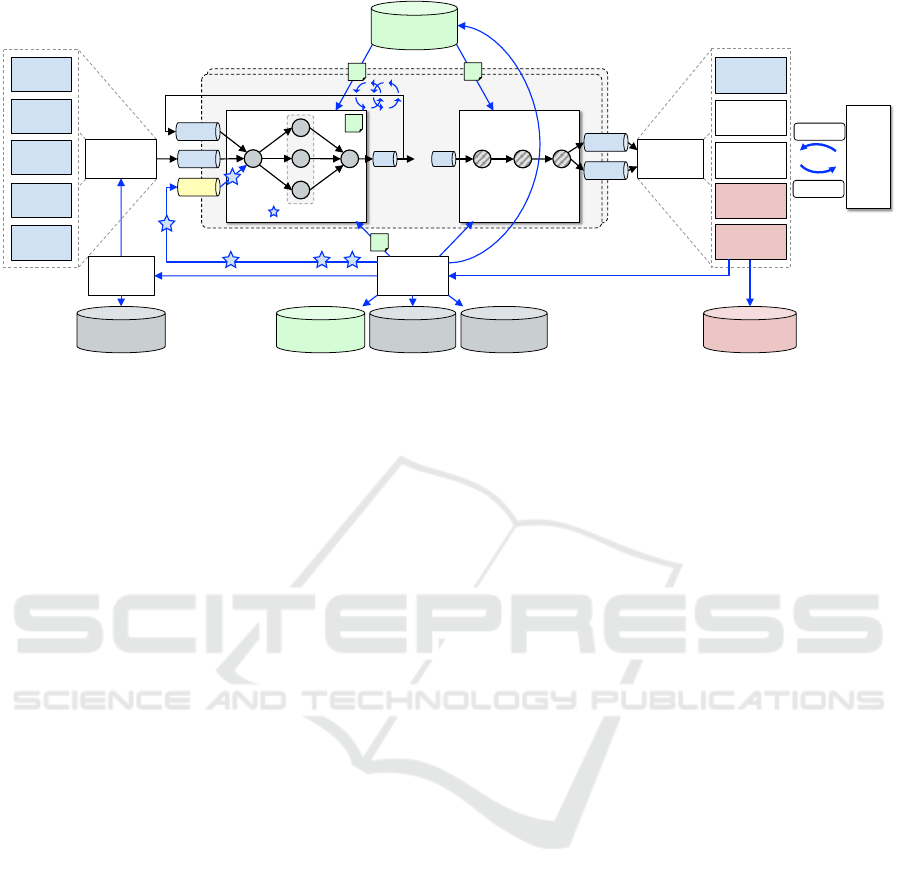
Figure 8: Conceptual Architectural Framework of BigGIS for performing spatio-temporal analytics at scale instantiating the
continuous refinement model (Wiener et al., 2016) during the exploration stage. Of particular note is that data flows (
→
),
moving from data sources to data sinks, are countercyclical to information/control flows (←) that originate from the user.
sented architectural elements (Def. 5 – pipelines, repos-
itories, services, user actions) interconnect and thus
instantiate the continuous refinement model (Wiener
et al., 2016) as shown in Figure 8. This, along with
the aforementioned requirements, form the basis of the
design considerations. A user interacting with BigGIS
would traverse through various stages during her anal-
yses. These stages are (1) preparation, (2) deployment,
and (3) exploration, that are discussed in the following.
5.1 Preparation
During the preparation stage, the user prepares for
data processing and analyses and either composes a
pipeline itself with the necessary nodes and configura-
tions from the node repository or utilizes a predefined
pipeline template from the pipeline repository for a
specific use case. While the former provides more flex-
ibility the latter further enables a set of suitable visual
analytics views from the visualization repository as a
designated data sink that allows for manipulation of
the processing nodes through refinement gate input
queues. Additional configuration of the node can be
made by the user in order to suit the needs. Configura-
tions are saved in the configuration repository by the
cognitive app service. Generally, the preparation stage
consists of data source and data sink selection as well
as pipeline composition and configuration.
5.2 Deployment
Once the configuration of the pipeline is completed
and the data sources and data sinks are specified, a user
action triggers the cognitive app service to deploy the
nodes on the underlying big data frameworks. Depend-
ing on wether the user has chosen a pipeline template,
the cognitive app service looks up the composition in
the pipeline repository, loads the appropriate nodes
and models from the corresponding repositories and
deploys them. Furthermore, the cognitive app service
triggers the linked API service to start the data integra-
tion process thereby leveraging the semantic annota-
tion and the rules of conversion from the data source
repository. The output of the data integration process
is published to specified queues from where it gets
consumed, continuously analyzed, refined and further
distributed to the selected data sinks. In this respect,
one eminent data sink type represents the aforemen-
tioned pipeline dependent visual analytics views. This
way, the results are presented in an adequate way that
enhances to cognitive and perceptive skills on user-side
to increase the likelihood of relevant findings during
the course of exploration.
5.3 Exploration
The exploration stage is characterized by two recurrent
steps, that involve (1) reasoning on interesting obser-
vations made by the user on retrieved results (finding),
e.g. missing data points, patterns in visual representa-
tions, or conspicuous predictions of machine learning
nodes and (2) manipulating the data processing or mod-
els (action). During the course of exploration, the user
constantly interacts with the visual analytics views to
understand the observations through certain elements,
e.g. adjusting parameters for a data heatmap layer
on top of OpenStreetMap data. This interactive user
action provokes the cognitive app service to update
the configurations and parameters in the configuration
repository and propagates refinement events (
F
) over
Taming the Evolution of Big Data and its Technologies in BigGIS - A Conceptual Architectural Framework for Spatio-Temporal Analytics
at Scale
99
Find
neighbour
Envisat pixels
!
c
1!
Stream Enrichment!
pipeline p
1!
Linked
API!
Cognitive
App!
Pipeline!
Repository!
Data Source!
Repository!
Data
Sources!
Envisat!
ATKIS!
weather
stations!
Visualization!
Repository!
Model!
Repository!
User!
Action!
Finding!
Human!Sources!
System!
Visual
Analytics!
Node!
Repository!
Data
Sinks!
Data
Storages!
Sinks!
Config!
Repository!
User Actions A!
Find inter-
sections with
ATKIS
polygons
!
c
2!
c
3!
Pick Top K
Land Use
Classes!
t=wstations
!
t=envisat
!
t=atkis
!
t=envisat-convolution
!
t=atkis-intersection
!
t=topk
!
t=topk-rgate
!
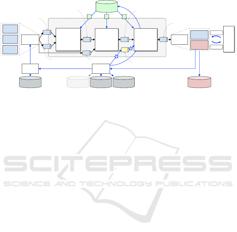
Figure 9: Stream Enrichment use case in BigGIS during the exploration stage showing three nodes and corresponding queue
topics t, as well as the relevant data sources and data sinks.
the refinement gate input queues to the designated
node instances. The node then updates its configura-
tion and parameters to satisfy the adjustments in order
for a fast retrieval of newly calculated results to allow
to continue reasoning on user-side. The continuous
refinement approach is especially beneficial in terms
of deployed machine learning nodes, where model pa-
rameters can be easily refined to improve the accuracy
of the prediction through (1) an iterative approach by
subscribing to the own output queue to automatically
supervise the process and autotune the parameters, as
well as (2) direct user involvement triggered by a re-
finement event. The latter can involve feedback in
types of corrections of predicted labels or parameters
itself. Eventually, new insights are generated when the
user is able to understand and interpret the findings in
the context of the problem domain.
6 DISCUSSION BY EXAMPLE
To discuss our framework, we formally show how the
Stream Enrichment use case from Section 3.3 is instan-
tiated within BigGIS as depicted in Figure 9, which
is presenting the running pipeline in the exploration
stage. Thus, the cognitive app service has already
read out the description of the corresponding stream
enrichment pipeline from the pipeline repository and
deployed the required nodes from node repository with
their specific configuration parameters on the underly-
ing big data infrastructure. Since there is no machine
learning involved in this use case, the model repository
is not active.
Overall, the stream enrichment pipeline consists
of three core nodes (Find neighbour Envisat pixels,
Find intersections with ATKIS polygons, Pick Top K
Land Use Classes), that are using a set of seven queues
(wtstation, envisat, atkis, envisat-convolution, atkis-
intersection, topk, topk-rgate). The input data sources
consists of (1) a data stream of sensor readings from
different types of weather stations (vector data), (2) En-
visat LST scans (raster data), as well as (3) ATKIS land
use classes (vector data). At the beginning, the sensor
readings need to be normalized based on a set of trans-
formations according to the semantic description in the
data source repository. Then, the normalized stream
is consumed by the first node in combination with the
latest Envisat LST scan of this region in order to find
the neighbour Envisat pixels and calculate the convolu-
tion. The second node uses this output and computes
the intersection with the land use class polygons of
this region from ATKIS. Lastly, the third node selects
the top-k land use classes and publishes them on a
dedicated output queue. From there, the enriched out-
put stream is stored in a database to persist the results
and is presented to the user in a visual analytics view,
thus allowing her to dictate top-k parameter changes to
the running pipeline through the refinement gate input
queue of the third node.
As shown in Table 1 the Stream Enrichment use
case does not involve batch processing or learning and
as consequence not all aspects of the use cases pre-
sented in Section 3 are discussed here in detail. How-
ever, with corresponding node design and/or pipe-line
self-subscription loop such capabilities are harmoni-
cally supported by our framework.
7 CONCLUSION AND FUTURE
WORK
In this paper, we have presented a conceptual archi-
tectural framework for spatio-temporal analytics at
GISTAM 2017 - 3rd International Conference on Geographical Information Systems Theory, Applications and Management
100

scale. The work is motivated by the big data induced
requirements in the field of geographic information
systems. Due to the constant progress particularly
in geoinformatics and the open source movement in
big data, a sustainable approach is necessary to pro-
tect previous investments in technologies and opera-
tional effort and to prepare for future developments.
The core challenges to sustainability that the archi-
tectural framework is facing are threefold: (1) hetero-
geneity of available data sources, (2) heterogeneity of
use cases as well as, (3) heterogeneity of the big data
landscape. These challenges are mainly addressed by
an integrated and unified approach that builds on the
established pipes and filters design pattern in combina-
tion with the continuous refinement model in BigGIS.
Our future work will on one hand focus on imple-
menting the proposed conceptual architectural frame-
work for the given uses cases and presenting these
incarnations. On the other hand we try to extend the
flexibility gained by the proposed architectural frame-
work from the conceptual to infrastructure level by
leveraging container technology for deployment and
management of BigGIS.
ACKNOWLEDGEMENTS
The project BigGIS (reference number: 01IS14012)
is funded by the Federal Ministry of Education and
Research (BMBF) within the frame of the research
programme “Management and Analysis of Big Data”
in “ICT 2020 – Research for Innovations”.
REFERENCES
Apache Foundation (2016). Apache NiFi Documentation.
https://nifi.apache.org/docs.html.
Berthold, M. R., Cebron, N., Dill, F., Gabriel, T. R., K
¨
otter,
T., Meinl, T., Ohl, P., Sieb, C., Thiel, K., and Wiswedel,
B. (2007). KNIME: The Konstanz Information Miner.
In Studies in Classification, Data Analysis, and Knowl-
edge Organization (GfKL 2007). Springer.
Buschmann, F., Henney, K., and Schmidt, D. C. (2007).
Pattern-Oriented Software Architecture – A Pattern
Language for Distributed Computing. John Wiley &
Sons, New York.
Crossland, M. D., Wynne, B. E., and Perkins, W. C. (1995).
Spatial Decision Support Systems: An Overview of
Technology and a Test of Efficacy. Decis. Support
Syst., 14(3):219–235.
Eclipse Foundation (2016). GeoTrellis Documentation.
http://geotrellis.io/documentation.html.
Emanuele, R. (2016). GeoTrellis landsat tutorial
project. https://github.com/geotrellis/geotrellis-landsat-
tutorial.
Esri (2016). ArcGIS and Big Data.
http://www.esri.com/products/arcgis-capabilities/big-
data/arcgis-and-big-data.
Guazzelli, A., Zeller, M., Lin, W., and Williams, G. (2009).
PMML: An open standard for sharing models. The R
Journal, 1(May):60–65.
Kreps, J. (2014). Questioning the Lambda Architec-
ture. https://www.oreilly.com/ideas/questioning-the-
lambda-architecture.
Marz, N. and Warren, J. (2013). Big Data: Principles
and Best Practices of Scalable Realtime Data Systems.
Manning Publications.
OGC (2013). Big Processing of Geospatial Data.
http://www.opengeospatial.org/blog/1866.
Ord, J. K. and Getis, A. (1995). Local spatial autocorrela-
tion statistics: Distributional issues and an application.
Geographical Analysis, 27(4):286–306.
Peng, Y. and Liangcun, J. (2014). BigGIS: How big data can
shape next-generation GIS. In 3rd Int. Conf. on Agro-
Geoinformatics (Agro-Geoinformatics 2014), pages
1–6. IEEE.
Riemer, D., Kaulfersch, F., Hutmacher, R., and Stojanovic,
L. (2015). Streampipes: Solving the challenge with
semantic stream processing pipelines. In Proc. of the
9th ACM Int. Conf. on Distributed Event-Based Sys-
tems, DEBS ’15, pages 330–331, New York, NY, USA.
ACM.
Sacha, D., Stoffel, A., Stoffel, F., Kwon, B. C., Ellis, G., and
Keim, D. A. (2014). Knowledge Generation Model for
Visual Analytics. IEEE Transactions on Visualization
and Computer Graphics, 20(12):1604–1613.
Thakur, G. S., Bhaduri, B. L., Piburn, J. O., Sims, K. M.,
Stewart, R. N., and Urban, M. L. (2015). PlanetSense:
A Real-time Streaming and Spatio-temporal Analytics
Platform for Gathering Geo-spatial Intelligence from
Open Source Data. In Proc. of the 23rd SIGSPATIAL
Int. Conf. on Advances in Geographic Information Sys-
tems, pages 11:1–11:4. ACM.
Tomlin, C. (1990). Geographic information systems and car-
tographic modeling. Prentice Hall series in geographic
information science. Prentice Hall.
Wiener, P., Stein, M., Seebacher, D., Bruns, J., Frank, M.,
Simko, V., Zander, S., and Nimis, J. (2016). BigGIS:
A Continuous Refinement Approach to Master Hetero-
geneity and Uncertainty in Spatio-Temporal Big Data
(Vision Paper). In 24th ACM SIGSPATIAL Int. Conf. on
Advances in Geographic Information Systems (ACM
SIGSPATIAL 2016).
Taming the Evolution of Big Data and its Technologies in BigGIS - A Conceptual Architectural Framework for Spatio-Temporal Analytics
at Scale
101
