Localization of Demyelinating Plaques in MRI using Convolutional

Neural Networks

Bartłomiej Stasiak

, Paweł Tarasiuk

, Izabela Michalska

, Arkadiusz Tomczyk

and Piotr S. Szczepaniak

Institute of Information Technology, Lodz University of Technology, Wolczanska 215, 90-924 Lodz, Poland

Department of Radiology, Barlicki University Hospital, Kopcinskiego 22, 91-153 Lodz, Poland

Keywords:

Multiple Sclerosis, Convolutional Neural Networks.

Abstract:

In the paper a method of demyelinating plaques localization in head MRI sequences is presented. For that

purpose a convolutional neural network is used. It is trained to act as non-linear ﬁlter, which should indicate

(give a high response) in those image areas where the sought objects are located. Consequently, the output

of the proposed architecture is an image and not a single label as it is in the case of traditional networks with

pooling and fully connected layers. Another interesting feature of the proposed solution is the ability to select

network parameters using smaller patches cut from training images which reduces the amount of data that

must be propagated through the network. It should be emphasized that the conducted research was possible

only thanks to the manually outlined plaques provided by radiologist.

1 INTRODUCTION

In recent years convolutional neural networks (CNN)

allowed to make a signiﬁcant progress in automatic

analysis of the images. It was possible thanks to the

technological progress (computations with GPU) and

access to large amount of labeled data. Labeled im-

age data, however, can be of different form. The most

popular (the easiest to gather) are data where the im-

age is accompanied by the label describing its con-

tent. This allows to train CNN solving a typical clas-

siﬁcation task. Other tasks, like precise localization

of objects (segmentation), require much more effort

to collect proper data. This task becomes even harder

if correct labeling of image content requires special-

ized, e.g. medical, knowledge. That is the case,

which is considered in this work where demyelinating

plaques are searched for within MRI (magnetic res-

onance imaging) data. The conducted research was

possible only thanks to the hard work of radiologist

who precisely outlined the regions of interest on ev-

ery slice of head MRI sequence.

As it was mentioned above, applying CNN to seg-

mentation task is not as popular as its application

to classiﬁcation problems. Two basic groups of ap-

proaches can be found in the literature. First one is

a patch based approach where labels are assigned not

to the whole image but to the selected regions of that

image (in particular to the regions representing neigh-

bourhood of a given pixel). In other words it is a mod-

iﬁed sliding window technique with CNN as a classi-

ﬁer. This classiﬁer, naturally, is not trained using the

whole image as an input. Instead, we use patches cut

from the training images, manually segmented by an

expert. Such a method was used, for example, in seg-

mentation of anatomical regions in MRI images (de

Brebisson and Montana, 2015). The second approach

uses a so-called fully convolutional approach (Shel-

hamer et al., 2016). In this case the whole image is

given as an input and as an output the image of the

same size, representing segmentation mask, is pro-

duced. To achieve such a functionality the network

has a special architecture. First some traditional con-

volutional and pooling layers are used, which reduces

the size of the resulting feature maps, and then some

upscaling (deconvolutional) layers are added to en-

large and combine those maps to obtain the image

of proper size. Such a fully convolutional network is

trained using whole images without the need of cut-

ting it into patches. This kind of approach was suc-

cessfully used in e.g. analysis of transmitted light

microscopy images (Milletari et al., 2016) and MRI

prostate examinations (Ronneberger et al., 2015). The

latter approach is particularly interesting since it con-

siders 3D convolution and the 3D MRI sequence is

processed by CNN as a whole.

Stasiak, B., Tarasiuk, P., Michalska, I., Tomczyk, A. and Szczepaniak, P.

Localization of Demyelinating Plaques in MRI using Convolutional Neural Networks.

DOI: 10.5220/0006298200550064

In Proceedings of the 10th International Joint Conference on Biomedical Engineering Systems and Technologies (BIOSTEC 2017) - Volume 2: BIOIMAGING, pages 55-64

ISBN: 978-989-758-215-8

The solution proposed in this work to some extent

possesses features of both those approaches. On one

hand, it tries to train CNN to act as a non-linear ﬁlter

capable of indicating areas of interest. Consequently

the output is the image of the same size as the input.

In this case, however, no pooling is used and conse-

quently no upscaling is required. On the other hand, it

allows to train such a network using smaller patches

without the necessity of processing as large amount

of data as needed for the training based on the whole

images.

The paper is organized as follows: the second

section describes the considered dataset and medical

background justifying the importance of demyelinat-

ing plaques localization, in the third section the pro-

posed method is discussed and in the fourth and the

ﬁfth section the obtained results and their analysis are

presented. Finally, the last section contains a short

summary of the conducted research.

2 MEDICAL BACKGROUND

Multiple sclerosis (MS) is a chronic autoimmune dis-

ease that attacks central nervous system and conse-

quently leads to neurological disability. The body’s

immune system destroys the nerve’s myelin sheaths

which form white matter in the brain and spinal cord.

The areas where the layer of myelin was damaged are

called demyelinating plaques and the whole is known

as demyelination. The diagnosis of the disorder is

made by the combination of clinical ﬁndings, the ex-

amination of cerebrospinal ﬂuid and MRI of the cen-

tral nervous system. In patients with clinical symp-

toms suggesting MS the brain MR imaging can show

multifocal white matter lesions which are plaques of

demyelination. Nevertheless the process of demyeli-

nation can be a part of many other disorders, it is not

speciﬁc only to MS. The diagnosis of MS is more

likely if the plaques are distributed in some typical

areas in the brain such as: around the lateral ventri-

cles (periventricular), especially while they are orien-

tated perpendicularly to the long axis of the ventricles,

in the corpus callosum, along the boundary between

the white matter and cortex, in the cerebral and cere-

bellar peduncles, pons and medulla oblongata. The

most useful MRI scans for identifying white matter

lesions are T2-weighted images (T2WI), particularly

FLAIR sequences (ﬂuid-attenuated inversion recov-

ery). On those images the demyelinating areas have

an abnormally high signal in comparison to the nor-

mal white matter. On T2WI both cerebrospinal ﬂuid

and white matter lesions present a high signal so the

contrast between them is rather poor. In FLAIR tech-

nique the signal of cerebrospinal ﬂuid is suppressed

what improves detecting of the white matter lesions,

especially in the periventricular distribution.

The present study has focused on marking the

lesions of demyelination on MR scans of the brain

(FLAIR sequences in axial plane). All magnetic reso-

nance images were obtained using 1,5 Tesla scanner.

The thickness of slices of each examination amounted

from 3mm to 5mm. The patient population consisted

of hundred people (ﬁfty men and ﬁfty women) of dif-

ferent age groups (between 19 and 66 years old). The

study has taken into consideration only patients with

conﬁrmed diagnosis of MS. The severity of the dis-

ease differed from newly diagnosed to longstanding

disorder. The plaques of demyelination on magnetic

resonance images were deﬁned as notable alterations

of the signal in the whole area occupied by the white

matter.

3 METHOD

Convolutional neural networks are typical solution to

the machine learning problems where the input data

has a structure of a ﬁnite-dimensional linear space

range. CNNs are biologically inspired (Hubel and

Wiesel, 1965) modiﬁcation of multilayer perceptron

(MLP) with reduced connections between layers and

extensive weights sharing. One of the most basic

properties is indifference to translation (LeCun and

Bengio, 1995). Unlike MLP, where any permutation

of inputs is equally useful for training, in CNNs the

structure of input data is important and remains pre-

served. Outputs of the hidden layers are called feature

maps (LeCun and Bengio, 1995; Cires¸an et al., 2011),

since they actually describe locations of the certain

features of the image. The CNN input is usually just

a raw digital image, with optional very basic pre-

processing (scaling, normalization, etc.) (Krizhevsky

et al., 2012).

The mentioned properties make CNNs useful for

feature extraction. The usual ﬁeld where CNNs are

used is image classiﬁcation – the state-of-art solu-

tions to the ImageNet Large Scale Visual Recogin-

tion Challenge (Deng et al., 2009) are based on CNNs

(Krizhevsky et al., 2012; Zeiler and Fergus, 2013;

Nguyen et al., 2015). However, there are related

works where CNN is used just as general-purpose fea-

ture extractor (Mopuri and Babu, 2015) or as a solu-

tion to the object localization problem (Matsugu et al.,

2003; Dai et al., 2014). Some deep and complex

CNNs trained for ILSVRC were also successfully ap-

plied as a part of larger solution to other image recog-

nition problems (Cheng et al., 2016). The usual ap-

BIOIMAGING 2017 - 4th International Conference on Bioimaging

∗

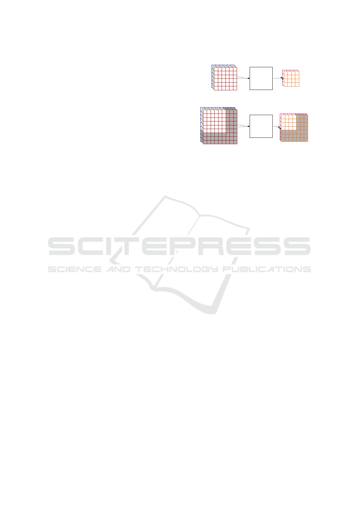
Input

(e.g. 3-channel

image)

Output: one matrix

for each group

of filters

∗

, A

1,1

, F

1,2

, F

1,3

2,1

, F

2,2

, F

2,3

, M

Figure 1: Convolutional layer internal structure. The exam-

ple setup processes A

, A

input with 2 groups of F

i, j

ﬁl-

ters (3 ﬁlters in each group). Convolution results produced

by each ﬁlter group are summed up. Each sum is a separate

output matrix, in this case: M

, M

proach expects the CNN to perform some dimension-

ality reduction of the input data, so the size of feature

maps in the consequent hidden layers is decreasing.

The reduced representation calculated with CNN is

usually used with some general-purpose classiﬁer –

MLP is preferred because of easy gradient learning of

the CNN+MLP classiﬁer as a whole (Cires¸an et al.,

2011).

Considering the structure of feature maps, it is

possible to perform a localization task, where the ex-

pected output is a feature map itself. It requires,

however, pure CNN architecture, without a classiﬁer,

since MLP breaks the topological image structure of

the hidden outputs. In order to get a map which could

be easily translated to object location on the input im-

age, we will ensure that the output size is the same as

input size. Instead of decreasing the size of the feature

maps, our approach involves simply keeping them

constant. Detailed application and consequences of

this approach are described in Section 3.2. By nor-

malization of the ﬁnal CNN output (e.g. with unipo-

lar sigmoid function) we produce a fuzzy map, where

each point is activated according to the likeliness of

belonging to the object. Further processing such as

noise removal and thresholding can be used to get the

binary mask, which is known to be useful in some ap-

plications (Dai et al., 2014). Similar remark applies

to the experiments performed in this work, as it is de-

scribed in Section 4.3. Our approach to thresholding

is presented in Section 3.3.

3.1 Formal Description

Let us denote the input data as a tuple of matrices

. . . A

of a ﬁxed n

× m

size (for the ﬁrst layer it

could be multi-channel digital image, or even a single

matrix for p = 1). The key parameters of a convo-

lutional layer (which is the basic unit of CNN) are

q ﬁlter groups – each of them being a tuple of p ma-

trices of n

× m

size (F

i, j

for i = 1 . . . p, j = 1 . . . q).

The output is a tuple of feature maps M

. . . M

where

for each i = 1 . . . q

= Z

∑

j=1

∗ F

i, j

In the formula above Z

is a bias matrix of the same

size as M

. Matrix convolution A

∗ F

i, j

is a matrix

of elements (A

∗ F

i, j

)

r,c

for r = 1 . . . (n

)−(n

)+1,

c = 1 . . . (m

)−(m

)+1 such that

∗ F

i, j

)

r,c

−1

∑

−1

∑

i, j

)

−d

),(m

−d

)

· (A

)

(r+d

),(c+d

)

The resulting M

matrices size is n

−n

+1×m

−

+1. Simpliﬁed diagram of convolutional diagram

is presented in Fig. 1.

Such a result could be easily processed further

with another convolutional layer. However, since the

matrix convolution with a ﬁxed F

i, j

is linear (and so

is the whole layer), it is advised to use some non-

linearity between the consequent convolutional lay-

ers. The obvious solution is to apply a non-linear ac-

tivation function element-wise. While sigmoid-like

function is known to work, the modern approach is

to use ReLU (rectiﬁed linear unit) (Krizhevsky et al.,

2012) or PReLU (parametrized extension of ReLU)

(He et al., 2015). The usual solutions for the clas-

siﬁer and feature extractor architectures additionally

use maximum- or average-pooling after some of the

convolutional layers. That approach reduces the ma-

trix dimensions by a certain factor (LeCun and Ben-

gio, 1995).

Each element of convolutional layer output is a re-

sult of processing some n

× m

rectangle picked

from each A

. For the ﬁrst feature map, n

× m

a size of visual ﬁeld (Hubel and Wiesel, 1965). For

further layers, the size of visual ﬁelds could be eas-

ily calculated by tracking down the range of CNN in-

put pixels affecting each output element. Should the

network consist of convolutional layers and element-

wise operations only, the visual ﬁeld size would

be n

× m

where n

= (n

+ . . . + n

) − t + 1 and

= (m

+ . . . + m

) −t + 1. In these formulas t de-

notes a number of convolutional layers and n

× m

is w-th layer ﬁlter size for w = 1 . . . t.

In our task, where it is desired to keep the orig-

inal size while processing with CNNs, pooling lay-

ers would be counterproductive. For any ﬁlters of

size other than 1 × 1 (which would perform just a

Localization of Demyelinating Plaques in MRI using Convolutional Neural Networks

point-wise combination), A

matrices have different

size than M

. To address that problem without any

change to the formulas, we can add padding to the A

which would increase the input size to (n

−1) ×

−1). Despite the size reduction of the orig-

inal layer, zero-padding can easily prevent any infor-

mation loss. Actually using padding of the proposed

size makes it possible to construct the identity opera-

tor, such as F

i, j

of odd dimensions with 1 in a central

element and 0 everywhere else. Another remark about

ﬂexibility of the proposed solution is that the padding

size (adding (n

−1) rows and (m

−1) columns) is

independent from the input size – it is related only to

the ﬁlter size.

3.2 Detector Training

Our proposed CNN architecture is a superposition of:

zero-padding (of a size which will keep the feature

map size constant) (LeCun et al., 1998), convolutional

layers and element-wise activation functions. We can

train such a network to in order to associate A

. . . A

with the resulting maps that represent the location of

objects. The location is described in the form of a

binary mask, which contains information about both

position and shape of the detected phenomena. Op-

timally the training images should include not only

the whole object, but some neighboring pixels of the

context as well.

If the object location on the image changes (but

context remains sufﬁcient), the CNN properties auto-

matically guarantee that we will get translated output.

It already makes application of CNN easier, than it

would be for a naive solution which would require

manual application of techniques such as sliding win-

dow. On related note, data augmentation through

small input translations is not necessary with CNNs.

The advantage of CNNs for the described sort of

tasks goes even further than that. Consider image

. . . B

, similar to A

. . . A

in all terms but size (it

still needs to be the same for each B

). It would be

especially practical if B

. . . B

is just a big image in-

cluding some objects to be detected. In some classi-

cal cases, external solutions such as sliding window

would be considered. Consider using B

. . . B

as an

input of our CNN. It could be remarked that:

• padding and convolution layer keep the image size

unchanged, since no parameters depend on input

size;

• convolution is still possible to calculate as long

as feature maps are larger than ﬁlters (which is

automatically satisﬁed if B

are larger than A

);

• element-wise functions are independent of the

map sizes as well.

Input

Output

, A

, M

CNN

, B

M’

, M’

Larger input

Extended output

Figure 2: Consider CNN like in Fig. 1. For each ad-

ditional row/column of input matrices, you get one more

row/column of the output. Case “a)” shows the original

setup. Consider variant “b)”, where the extended input is

used. If you choose a rectangle of the same size as A

ma-

trices, some outputs produce results similar to the “a)” setup

(e.g. it would work that way for the pixels of B

and M

dis-

played in white).

The output map would still show the proper mask

of a detected object (Dai et al., 2014), since it was

invariant to translation anyways. Without any addi-

tional utilities – after training on the small samples

(which is remarkably faster than processing a big im-

age with a small object) we get an object detector with

support of any greater input size, as it is shown in

Fig. 2. Detecting multiple objects works out of the

box as well. If there is some space between the ob-

jects to detect, so the visual ﬁelds do not intersect, the

process becomes equivalent to the detection of a sin-

gle object.

In order to avoid noise related to the “unknown”

input ranges appearing in the bigger image, our train-

ing set includes negative samples as well, as it is de-

scribed in Section 4.1. Using some context around the

object in the input images already prevents CNN from

picking any points of the included background, but

it leaves the network unprepared for any phenomena

that occur only in greater distance from the detected

objects.

Application of the mentioned methods for de-

myelinating plaques localization is explained further

in Sections 4.1-4.3.

3.3 Evaluation

As mentioned above, the size of the feature maps

is kept constant from layer to layer in the proposed

neural network. We also do not use MLP layers at

the output and the goal of the training is regression

rather than classiﬁcation. Putting the raw MR scan

BIOIMAGING 2017 - 4th International Conference on Bioimaging

on the CNN input we expect that the output consists

of the same-sized image, clearly marking the MS le-

sions as white regions, surrounded by black, neutral

background. In practice, however, the output image

will not be truly black-and-white, and the intensity

of a given output pixel may be interpreted rather in

terms of the probability that it is a part of a lesion.

Therefore, we have to apply thresholding to make the

ﬁnal decision and to obtain a black-and-white result

that may be directly compared to the expert-generated

ground-truth mask.

The value of the threshold is the fundamental pa-

rameter enabling to control the two elementary mea-

sures of the quality of the results: precision and recall.

Both these measures are based on the count of the

“true-positive” pixels in the CNN output image, i.e.

the pixels with values exceeding the threshold (“pos-

itive”), which at the same time represent the true MS

lesions, as indicated by the ground-truth masks. Re-

call is deﬁned as the proportion of the “true-positive”

pixels to all of the pixels that should be detected (ac-

cording to the mask) and precision is the proportion

of the “true-positive” pixels to all actually detected

pixels. Obviously, low threshold maximizes the re-

call and high threshold maximizes the precision. Ex-

tremely low threshold would render all the pixels pos-

itive, yielding 100% recall and close-to-zero preci-

sion, while extremely high threshold would do the

opposite. Therefore, a standard approach to obtain

a representative results, applied also in our approach,

is to compute the harmonic mean of precision and re-

call, known as F-measure.

The value of F-measure is used in the evaluation

of the obtained results to ﬁnd the appropriate thresh-

old. We apply a search through all possible thresh-

old values, recording the resulting F-measure values

for the training images. The threshold maximizing

the F-measure is used to compute the ﬁnal results on

a separate set of testing images, as described in the

following section.

4 EXPERIMENTS

4.1 Dataset Preparation

From the initial set of 100 patients, 4 were removed

from the study due to MR image format discrepan-

cies. The remaining 96 were split at random into the

training set (77 patients) and the testing set (19 pa-

tients). Each patient was represented by a set of MR

scans of the size 448×512 pixels, out of which only

the scans containing plaques of demyelination were

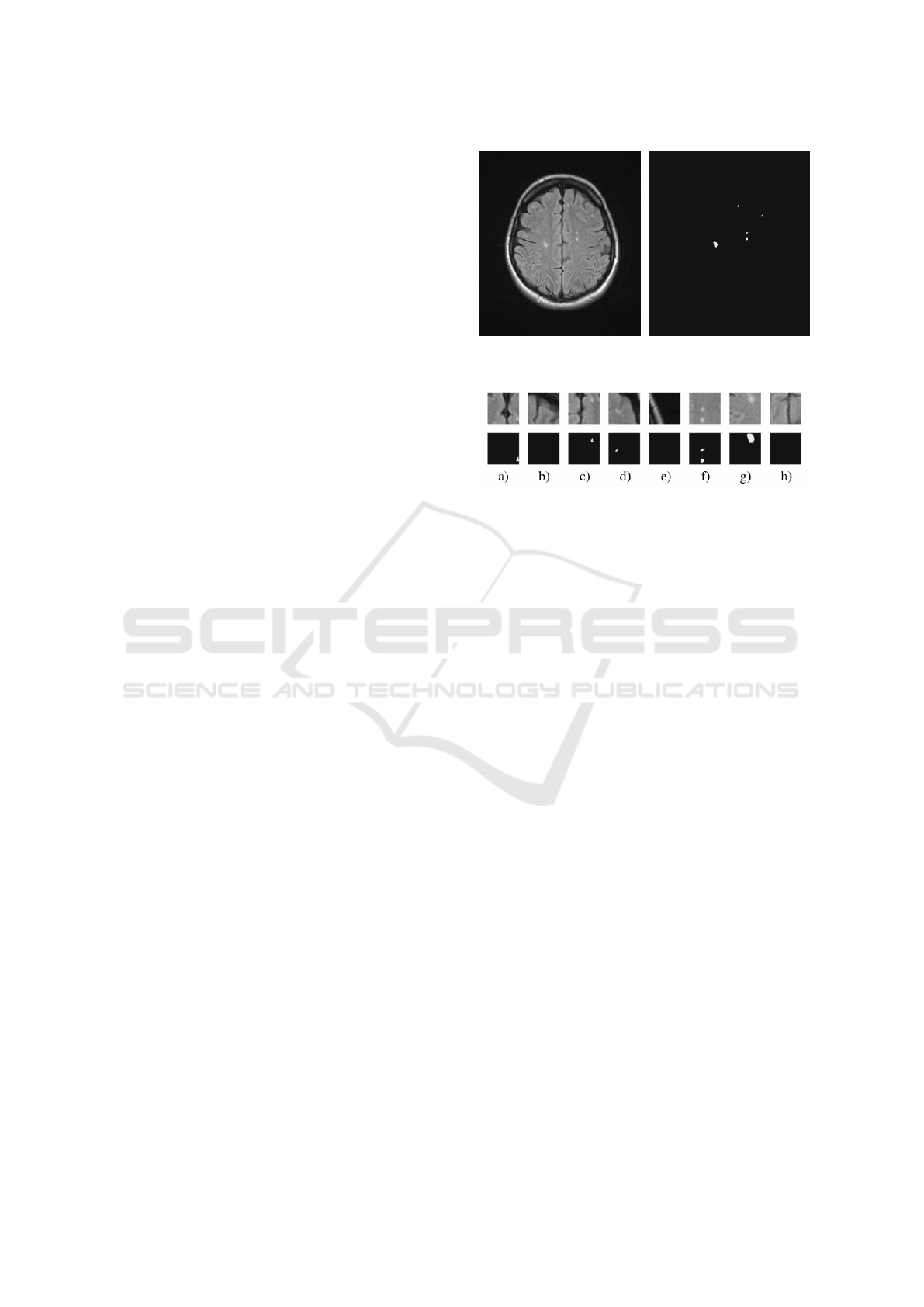
Figure 3: Example of a scan used in the training set (left)

and the accompanying mask (right).

Figure 4: Example of tiles cut from the scan in Fig. 3 (top)

and the accompanying masks (bottom). Note, that tiles b),

e), h) do not contain lesions and that tiles a) and c) represent

the same (topmost) lesion.

considered. As a result, the testing set contained 242

scans and the training set was based on 982 scans.

In the latter case however, the 982 scans were not

directly used but they were cut into tiles of 50×50

pixels and only some of them were selected for in-

clusion into the ﬁnal training set. Basically, the se-

lected tiles were all those containing demyelinations.

However, preliminary tests revealed that in this way

some parts of the scans, such as the skull bones, areas

around eye globes and sinuses, were never included

in the training set. As an effect, they were usually

mistakenly marked as demyelinations on the testing

set, as they were typically brighter than the surround-

ing regions, similarly to the MS lesions. Therefore, to

let the neural network learn and recognize these areas

and to decrease the risk of false alarms, some of the

tiles without lesions were also included in the training

set (Fig. 3 and Fig. 4). These tiles were selected at

random, but with some additional constraints giving

preference to bright areas and high contrast. Out of

the total number of 7856 tiles constituting the training

set, approximately one-third were these “no-lesion”

tiles. The last operation performed on the tiles with

lesions was to detect when a lesion occurred at the

edge of the tile so that only a part of it was included.

In such cases the tile was shifted appropriately to in-

crease the chance of encompassing the whole lesion.

Localization of Demyelinating Plaques in MRI using Convolutional Neural Networks

4.2 CNN Architecture

The structure of the network, i.e. the number of lay-

ers, the number of neurons, the size of the receptive

ﬁelds and the non-linearity types were the subject of

intensive experiments in our study. The ﬁnal archi-

tecture, offering the possibility of successful training

and moderate generalization error is composed of 6

convolutional layers:

• 20 neurons (5×5, padding: 2)

• 20 neurons (7×7, padding: 3)

• 40 neurons (9×9, padding: 4)

• 60 neurons (7×7, padding: 3)

• 20 neurons (5×5, padding: 2)

• 1 neuron (5×5, padding: 2)

We applied parametric rectiﬁed linear units (PReLU)

between the layers, and after the last layer the unipo-

lar sigmoid was used.

4.3 Testing Procedure and Results

The experiments were done with Caffe deep learning

framework on a cluster node with Tesla K20M GPU

accelerator. The training set of 7856 50×50 tiles was

fed to the network in mini-batches of 100 tiles each.

Mean square error (Euclidean loss) between the net-

work outputs and the ground-truth masks was used as

the indicator of the training progress.

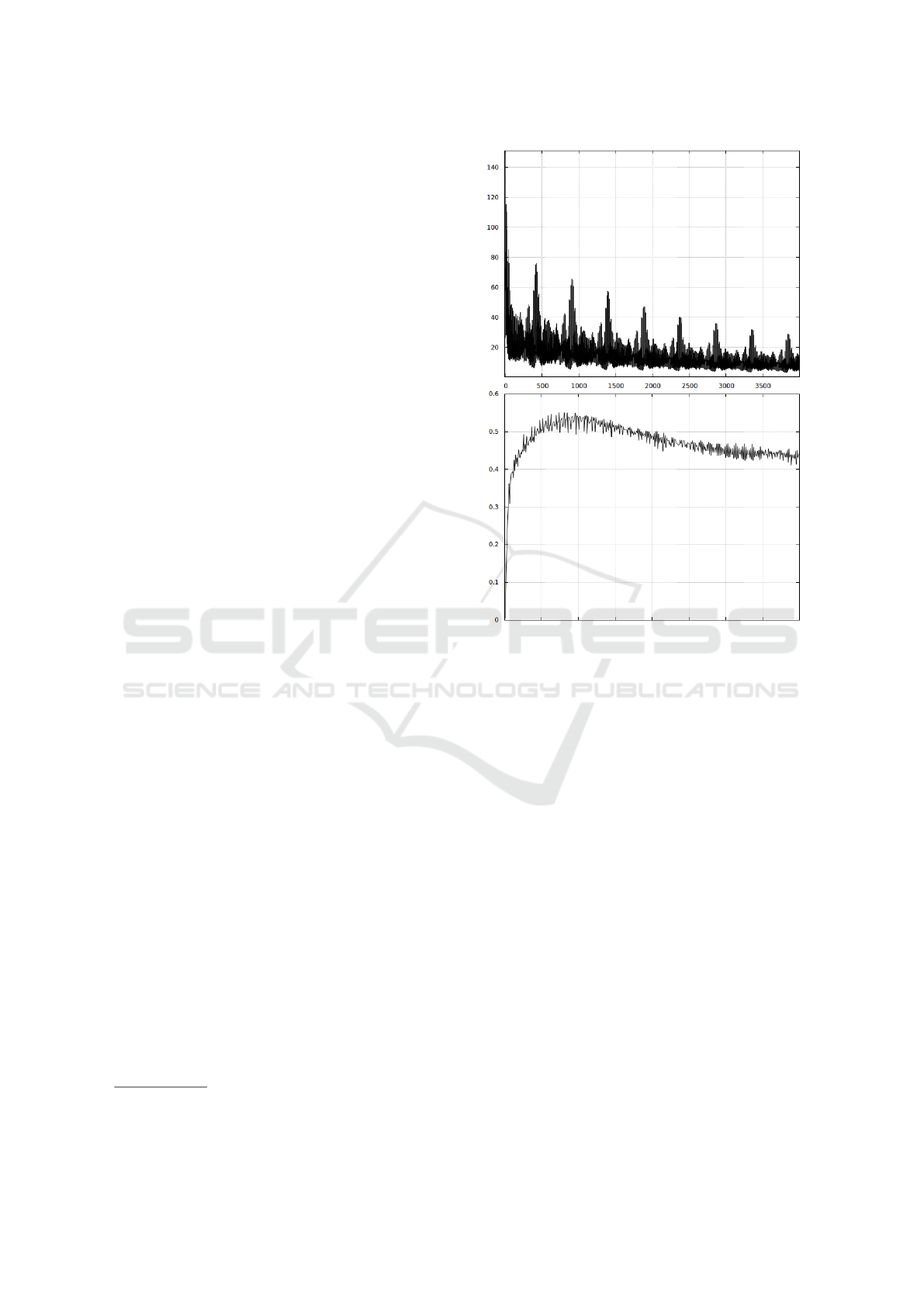
After several experiments with various parame-

ters of the learning process, we set the initial learn-

ing rate and momentum to 0.00001 and 0.9, respec-

tively. These values guaranteed slow but stable con-

vergence, as demonstrated in Fig. 5 (top plot). The

decrease of the error is clearly visible, which indicates

that the network learns to detect lesions on the train-

ing tiles. It appeared, however, that the enhancement

of the resulting F-measure value was observed only

during the initial phase of the training, as evidenced in

the bottom plot of Fig. 5. We have therefore a typical

problem of generalization error, increasing when the

network is getting overtrained. It should be stressed,

however, that the presented plots correspond to ca. 80

hours of learning, during which the whole training set

was used over 5000 times. It is also worth to note, that

the period of the visible cycles encompasses exactly

625 repetitions of the whole training set

In the following part, we will demonstrate the

practical effectiveness of the network trained for the

optimal time (ca 15 hours), using the full MR scans

This number results from the relation between the size

of the mini-batch and the number of tiles in the training set.

Figure 5: Top: learning curve (Euclidean loss); bottom:

F-measure on the testing set. The unit on the horizontal

axis corresponds to 100 mini-batches (each containing 100

tiles).

448×512 from the testing set. It is worth noting here,

that our CNN composed of convolutional layers only

(no MLP layers) behaves more like an image ﬁlter,

accepting any size of the input image without the

need of architecture changes or re-adaptation of the

weights, as pointed out in Section 3.2. This is a sig-

niﬁcant advantage of our approach, enabling to use

full scans to test the network trained on small tiles.

In order to practically verify the effectiveness of

the network on the testing set, we thresholded the net-

work output to obtain the binary image for direct com-

parison with the mask. The value of the threshold was

set so that it maximized the F-measure on the training

set, as described in Section 3.3. It appeared, however,

that the characteristics of the training set composed

of small tiles, was so different from the testing set

containing full scans, that the obtained threshold val-

ues were unsuitable for the use in the testing phase.

Therefore we decided to use the original training im-

ages to compute the threshold. In short, the training

images were used in two forms: cut into tiles (7856

tiles) for network training and uncut (982 scans) for

BIOIMAGING 2017 - 4th International Conference on Bioimaging

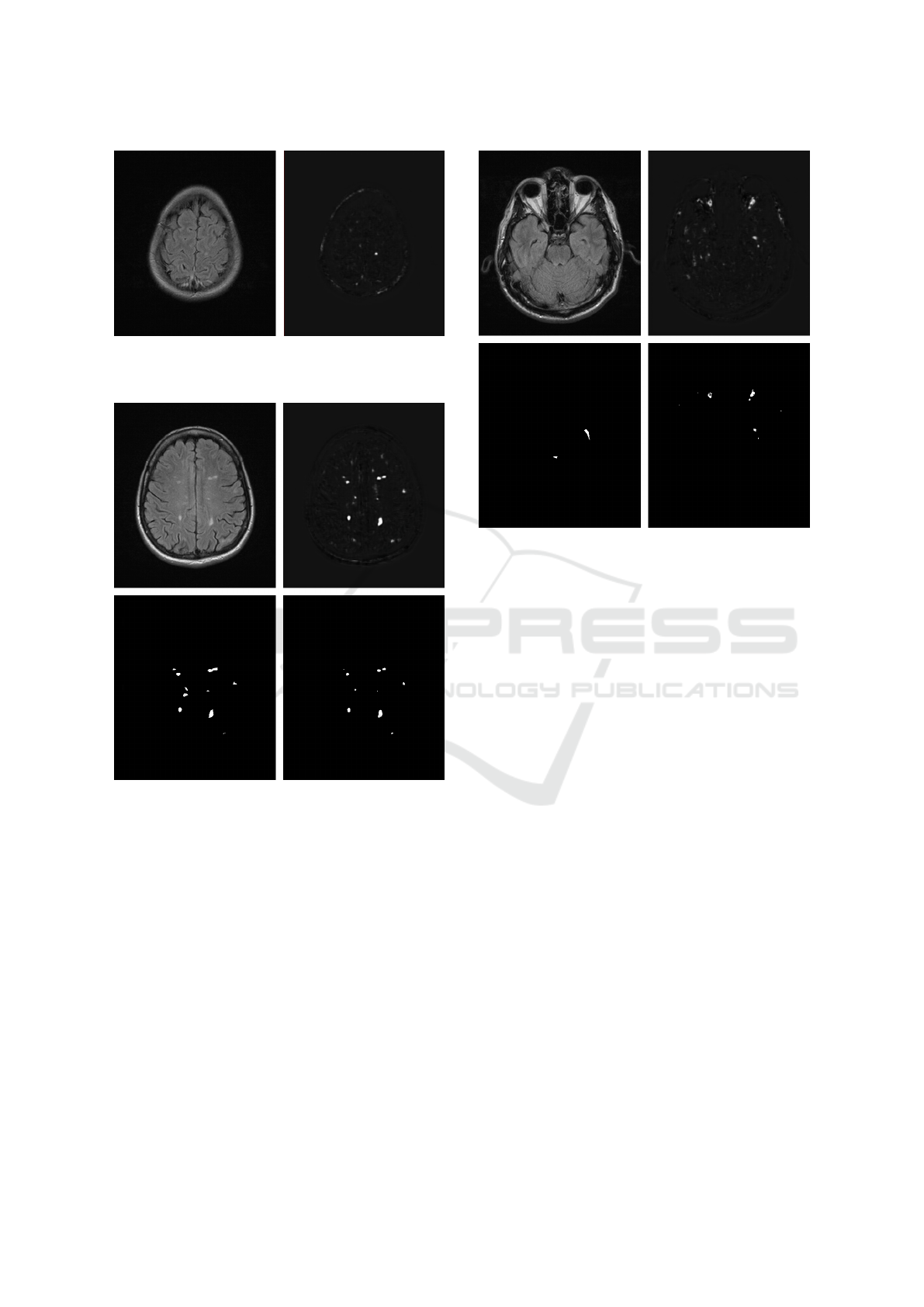
Figure 6: Example of input (left) and output (right) of the

network – a single lesion in the right hemisphere was prop-

erly indicated.

Figure 7: Left column: input image (top) and ground truth

mask (bottom); right column: CNN output image before

thresholding (top) and after thresholding (bottom).

threshold determination.

An example of the results obtained on the testing

set after training is presented in Fig. 6. The image on

the right presents raw network output before thresh-

olding, which in this case, enabled to perfectly de-

tect the demyelination region in the right hemisphere.

It should be noted that this lesion is not very salient

in the input image, which contains many brighter re-

gions, such as the bottom of the hemispheres and the

skull bones. The network actually performs as an

image ﬁlter, amplifying the signal in the regions re-

sembling those learned during training, irrespective

of their absolute brightness.

Fig. 7 presents a more complicated case with

many lesions which has also been detected (all except

Figure 8: Left column: input image (top) and ground truth

mask (bottom); right column: CNN output image before

thresholding (top) and after thresholding (bottom).

one in the left hemisphere). In Fig. 8, however, sev-

eral signiﬁcant problems are revealed, including false

alarms for the tissue surrounding the optic nerves and

the temporal bones. Out of the two genuine lesions

only one is found and unnecessarily split into two dis-

joint regions.

5 ANALYSIS

The examples presented in the previous section give

an idea of what can be expected from our CNN af-

ter training. These results are promising in that they

demonstrate the network’s ability to detect typical de-

myelination lesions. What is important, this ability

seems to be based not only on their intensity but also

on their shape and characteristics of the surrounding

tissue. For comparison, let us consider a simple ap-

proach based on direct thresholding of the raw input

image. An example for the same image as in Fig. 6 is

presented in Fig. 9. As we may observe, the thresh-

old of 50% is too low to correctly detect the lesion,

whereas the number of false positive areas is signif-

icant and it rises dramatically even with quite mod-

erate decrease of the threshold. Clearly, irrespective

on the threshold, the result is virtually useless. On

the other hand, the CNN output presented in Fig. 6

(the image on the right) may be thresholded yielding

the correct outcome, i.e. a single region in the appro-

Localization of Demyelinating Plaques in MRI using Convolutional Neural Networks

Figure 9: Example of thresholding of the raw input image

from Fig. 6 with threshold values 50%, 45% and 40% (from

left to right, respectively).

priate location, for a wide range of threshold values

(from 48% to 92% in this particular case).

Considering the overall results it should be noted,

however, that the obtained F-measure values reach

only 55% in the best cases (Fig. 5, bottom) which can-

not be generally deemed a successful outcome. There

are a few sources of this and we will now try to inves-

tigate them in more detail and to formulate possible

solutions.

The ﬁrst problem, already addressed in Sec-

tion 4.1 is related to the structures adjacent to the

tissues of the central nervous system, such as bones,

meninges and sinuses. They are basically out of the

scope of our study, but they are nevertheless present

in the MR scans so we attempted to purposely train

the CNN to ignore them, as described above. This

attempt was mostly successful, as demonstrated in

Fig. 6 and 7, but it tends to fail in a case when these

structures contain bright regions of considerable size

(Fig. 4). This problem is particularly pronounced in

the topmost MR scans where the bones of the calvaria

are not perpendicular to the projection plane, so they

appear much broader.

There are several possible solutions here, includ-

ing the increase of the number of tiles representing

such structures in the training set, to make the net-

work recognize them better. Another important rem-

edy would also be to increase the size of the tiles.

The 50×50 tiles may be simply too small to incor-

porate enough surrounding tissues in case of bright

regions of signiﬁcant size. However, both these coun-

termeasures lead to increase of the area without le-

sions in the ground-truth masks. This in turn may

make the network learn to generate purely black out-

put images, because the associated local minimum of

the error function would not differ much from the de-

sired learning goal. The ultimate solution is therefore

to use some automatic or semi-automatic tools to re-

move the irrelevant parts of the input MR scans prior

to CNN training and testing. This would be less uni-

versal, but it would let the CNN concentrate on the

regions of interest (cerebral tissue) only.

The second issue negatively inﬂuencing the ob-

tained results is the quality and the quantity of the ma-

terial available for training. Most of the demyelinat-

ing plaques are unambiguously visible in the scans,

but still there are also many small or very faint lesions

which may pose problems in unequivocal identiﬁca-

tion as MS plaques. The problems with generaliza-

tion, indicated in Fig. 5, may suggest that we should

use a signiﬁcantly bigger set of training images or

more consistently annotated, perhaps by several in-

dependent specialists.

Yet another problem is associated with the preci-

sion of deﬁning the boundaries of the lesions by hu-

man annotators. Quite a signiﬁcant impact on the

quality of the obtained results stems from the fact

that even if all the lesions were properly detected in

the output image, they typically differ in size and

shape from the ground-truth masks. Due to this fact,

a different approach to the assessment of the out-

comes might be applied: instead of simply count-

ing the matching/non-matching pixels we might only

consider whether a lesion has been detected or not.

This would need some more effort for ﬁnding the con-

nected components in the masks and in the thresh-

olded output images, handling the splitting/joining of

adjacent lesions, etc. but evaluation generated in this

way would more accurately reﬂect the true usefulness

of the obtained results.

6 CONCLUSIONS AND FUTURE

WORK

Careful analysis of brain MRI is an important, time-

consuming part of MS diagnosis. While the ﬁnal de-

cision on interpretation belongs to the human expert,

artiﬁcial intelligence can provide tools that assist the

analysis process. Manual detection and localization

of demyelinating plaques visible on MRI is expected

to be unambiguous, but there is no concise mathemat-

ical formula to describe a plaque. The objective of our

work is to get the best suggestions from the convolu-

tional neural network.

The collected dataset included MRI scans of 100

patients of different age groups. Multiple slices were

stored as relatively large digital images (448 × 512

pixels). Cutting large images into 50 × 50 training

set tiles allowed us to perform the CNN training from

scratch. Due to the CNN properties described in Sec-

tion 3.2, the resulting network supported larger im-

ages out-of-the-box.

In order to compare the result to the target binary

masks properly, a mechanism of automatic threshold-

ing was designed, as it was described in Section 3.3.

As the evaluation was reduced to the comparison of

BIOIMAGING 2017 - 4th International Conference on Bioimaging

output and target binary masks, we could directly cal-

culate precision, recall and F-measure.

The best of the proposed models provided F-

measure of 55% on the test set. This value itself

is way from the perfect score. However, getting the

general location of the plaque and slightly imprecise

shape already reduces the value below 100%. The

gold standard consisted of approximate polygons, so

repeating it precisely is virtually impossible. More

signiﬁcantly problematic factors were related to the

false positives at the large bright areas, such as overly

activated points near the temporal bones and optic

nerves. Another common source of errors was re-

lated to mistakenly activated small regions (noise un-

related to the demyelinating plaques). On the other

hand, presence of selected points in the general area

of demyelinating plaques is a notable advantage of the

suggested model.

This result leaves much room for improvement.

Larger data set, which would include greater vari-

ety of cases, is expected to improve the results. Us-

ing 50 ×50 tiles could be considered disadvantageous

when compared to larger tiles, based on assumption

that larger visual ﬁelds could make it easier to recog-

nize temporal bones and optical nerves. However, the

initial tests on larger tiles resulted in all-zero network

outputs, because great majority of target outputs was

black. This problem would have to be addressed by

some speciﬁc approach such as cost function modiﬁ-

cation. Another solution could involve creating a sep-

arate tool to remove the irrelevant parts from the im-

age – which means everything besides the brain itself,

where myelin sheath of neurons is visible.

Using convolutional neural networks for medical

image processing is usually difﬁcult because of lim-

ited sizes of data sets. This common problem occured

to our work as well. However, our analysis is a step

towards more efﬁcient solutions. Our approach to the

dynamic threshold selection and chosen measure of

localization correctness (F-measure of the binary ma-

trix) will be useful for testing the future models.

The solutions mentioned above are mostly slight

improvements to the researched method. Another

possible way of the future work involves using pre-

trained CNNs as a part of the model. This is likely

to involve very complex and general solutions such

as AlexNet (Krizhevsky et al., 2012) or VGG (Si-

monyan and Zisserman, 2014). Despite the original

objective of those networks, which is classiﬁcation,

crucial parts of the same models could be used for

localization as well. Apparently, classiﬁcation and lo-

calization with CNNs are vastly similar tasks, and one

training process could result in an integrated solution

to both of them (Sermanet et al., 2013). The presence

of the pooling layers results in lower output mask res-

olution. This problem, however, could be addressed

with deconvolutional neural networks (Zeiler and Fer-

gus, 2013).

ACKNOWLEDGEMENTS

This project has been partly funded with support from

National Science Centre, Republic of Poland, deci-

sion number DEC-2012/05/D/ST6/03091.

Authors would like to express their gratitude to the

Department of Radiology of Barlicki University Hos-

pital in Lodz for making head MRI sequences avail-

able.

REFERENCES

Cheng, G., Zhou, P., and Han, J. (2016). Learning rotation-

invariant convolutional neural networks for object de-

tection in vhr optical remote sensing images. IEEE

Transactions on Geoscience and Remote Sensing,

54(12):7405–7415.

Cires¸an, D. C., Meier, U., Masci, J., Gambardella, L. M.,

and Schmidhuber, J. (2011). Flexible, high perfor-

mance convolutional neural networks for image clas-

siﬁcation. In Proceedings of the Twenty-Second Inter-

national Joint Conference on Artiﬁcial Intelligence -

Volume Volume Two, IJCAI’11, pages 1237–1242.

Dai, J., He, K., and Sun, J. (2014). Convolutional fea-

ture masking for joint object and stuff segmentation.

CoRR, abs/1412.1283.

de Brebisson, A. and Montana, G. (2015). Deep Neural

Networks for Anatomical Brain Segmentation. ArXiv

e-prints, 1502.02445.

Deng, J., Dong, W., Socher, R., Li, L.-J., Li, K., and Fei-

Fei, L. (2009). ImageNet: A Large-Scale Hierarchical

Image Database. In CVPR09.

He, K., Zhang, X., Ren, S., and Sun, J. (2015). Delving deep

into rectiﬁers: Surpassing human-level performance

on imagenet classiﬁcation. CoRR, abs/1502.01852.

Hubel, D. H. and Wiesel, T. N. (1965). Receptive ﬁelds and

functional architecture in two nonstriate visual areas

(18 and 19) of the cat. Journal of Neurophysiology,

28:229–289.

Krizhevsky, A., Sutskever, I., and Hinton, G. E. (2012).

Imagenet classiﬁcation with deep convolutional neu-

ral networks. In Pereira, F., Burges, C. J. C., Bottou,

L., and Weinberger, K. Q., editors, Advances in Neu-

ral Information Processing Systems 25, pages 1097–

1105. Curran Associates, Inc.

LeCun, Y. and Bengio, Y. (1995). Convolutional networks

for images, speech, and time-series. In Arbib, M. A.,

editor, The Handbook of Brain Theory and Neural

Networks. MIT Press.

LeCun, Y., Bottou, L., Bengio, Y., and Haffner, P. (1998).

Gradient-based learning applied to document recogni-

tion. In Proceedings of the IEEE, pages 2278–2324.

Localization of Demyelinating Plaques in MRI using Convolutional Neural Networks

Matsugu, M., Mori, K., Mitari, Y., and Kaneda, Y.

(2003). Subject independent facial expression recog-

nition with robust face detection using a convolutional

neural network. Neural Networks, 16(5-6):555–559.

Milletari, F., Navab, N., and Ahmadi, S.-A. (2016). V-

Net: Fully Convolutional Neural Networks for Vol-

umetric Medical Image Segmentation. ArXiv e-prints,

1606.04797.

Mopuri, K. R. and Babu, R. V. (2015). Object level

deep feature pooling for compact image representa-

tion. CoRR, abs/1504.06591.

Nguyen, T. V., Lu, C., Sepulveda, J., and Yan, S. (2015).

Adaptive nonparametric image parsing. CoRR,

abs/1505.01560.

Ronneberger, O., Fischer, P., and Brox, T. (2015). U-Net:

Convolutional Networks for Biomedical Image Seg-

mentation. ArXiv e-prints, 1505.04597.

Sermanet, P., Eigen, D., Zhang, X., Mathieu, M., Fergus,

R., and LeCun, Y. (2013). Overfeat: Integrated recog-

nition, localization and detection using convolutional

networks. CoRR, abs/1312.6229.

Shelhamer, E., Long, J., and Darrell, T. (2016). Fully

Convolutional Networks for Semantic Segmentation.

ArXiv e-prints, 1605.06211.

Simonyan, K. and Zisserman, A. (2014). Very deep con-

volutional networks for large-scale image recognition.

CoRR, abs/1409.1556.

Zeiler, M. D. and Fergus, R. (2013). Visualizing

and understanding convolutional networks. CoRR,

abs/1311.2901.

BIOIMAGING 2017 - 4th International Conference on Bioimaging