
Predicting Outcome of Ischemic Stroke Patients using Bootstrap
Aggregating with M5 Model Trees
Ahmedul Kabir
1
, Carolina Ruiz
1
, Sergio A. Alvarez
2
and Majaz Moonis
3
1
Dept. of Computer Science, Worcester Polytechnic Institute, 100 Institute Road, Worcester, MA 01609, U.S.A.
2
Dept. of Computer Science, Boston College, Chestnut Hill, MA 02467, U.S.A.
3
Dept. of Neurology, Univ. Massachusetts Medical School, Worcester, MA 01655, U.S.A.
Keywords: Ischemic Stroke, mRS Score, M5 Model Tree, Bootstrap Aggregating, Predicting Stroke Outcome.
Abstract: The objective of our study is to predict the clinical outcome of ischemic stroke patients after 90 days of
stroke using the modified Rankin Scale (mRS) score. After experimentation with various regression
techniques, we discovered that using M5 model trees to predict the score and then using bootstrap
aggregating as a meta-learning technique produces the best prediction results. The same regression when
followed by classification also performs better than regular multi-class classification. In this paper, we
present the methodology used, and compare the results with other standard predictive techniques. We also
analyze the results to provide insights on the factors that affect stroke outcomes.
1 INTRODUCTION
Stroke is defined as the rapid loss of brain function
caused by disturbances in the blood supply to the
brain. It is one of the leading causes of death
worldwide (Raffeld et al., 2016). Stroke can be
broadly classified into two types: Ischemic, which
occurs due to lack of blood flow; and hemorrhagic,
which is caused by internal bleeding. In this study
we deal with data from patients with ischemic stroke
which is the more common of the two types,
accounting for around 87% of all strokes
(Mozaffarian et al., 2016). The data are collected
retrospectively from the University of Massachusetts
Medical School, Worcester, Massachusetts, USA
and comprise demographic information, medical
history and treatment records of 439 patients.
The objective of this study is to predict the
outcome of a stroke patient in terms of the modified
Rankin Scale (mRS) score, an integer value between
0 and 6 measuring the degree of disability or
dependence in daily activities of people who have
suffered a stroke (Rankin, 1957). There are two
approaches one may use to solve this problem. One
is to treat the target as a numeric attribute and apply
some form of regression. The other approach would
be to think of the several different mRS scores as
different categories, in which case the problem
becomes that of multi-class classification. We have
addressed the prediction task from both perspectives.
1.1 Scope of this Paper
In this paper, we aim to predict the mRS score of a
patient after 90 days of an ischemic stroke based on
the data we have about the patient at the time of
discharge. Knowledge gained from this prediction
task may help medical practitioners manage stroke
more effectively and allocate resources more
efficiently. The predictive (or independent) attribu-
tes in our study consist of demographic information,
medical history and treatment records. The target
attribute is mRS-90, the mRS score at 90 days
following stroke onset (described in Table 1). We
treat the target as a numeric attribute first and apply
different regression techniques for prediction. Our
studies show that M5 model trees used in tandem
with bootstrap aggregating (bagging) significantly
outperforms other common regression methods such
as linear regression. We then treat the target as a
multiclass categorical attribute and apply several
classification techniques. Classification using the
aforementioned regression technique followed by
translation of the target to a discrete value performs
better than well-known classification methods such
as logistic regression and C4.5 decision trees.
178
Kabir A., Ruiz C., Alvarez S. and Moonis M.
Predicting Outcome of Ischemic Stroke Patients using Bootstrap Aggregating with M5 Model Trees.
DOI: 10.5220/0006282001780187
In Proceedings of the 10th International Joint Conference on Biomedical Engineering Systems and Technologies (BIOSTEC 2017), pages 178-187
ISBN: 978-989-758-213-4
Copyright
c
2017 by SCITEPRESS – Science and Technology Publications, Lda. All rights reserved

1.2 Modified Rankin Scale
The modified Rankin Scale (mRS) measure is the
most widely used clinical outcome measure for
stroke. It was first introduced by Dr. John Rankin
(Rankin, 1957) and later modified to its current form
by a group of researchers during the late 1980s (Van
Swieten et al., 1988). The mRS score is an integer
between 0 and 6 signifying the various degrees of
impairment caused by stroke, with 0 being the least
amount of impairment and 6 being death. Table 1
presents a summary description of the different mRS
scores. The mRS score can be calculated at various
stages of stroke. In this study, the mRS scores are
recorded in three different stages. The first, mRS
before admission, presents the degree of disability
the patient had before the onset of stroke. The next is
mRS at discharge, which gives the mRS score at the
time the patient is discharged from the hospital after
initial treatment of stroke. The last one is mRS at 90
days after stroke (mRS-90), the score this study
attempts to predict.
Table 1: Different mRS scores and their description
(Banks and Marotta, 2007).
Score Description
0 No symptoms
1 No significant disability
2 Slight disability
3 Moderate disability: requires assistance
4 Moderately severe disability
5 Severe disability: patient bedridden
6 Death
1.3 Related Work
The mRS-90 score has been used as a measure of
stroke outcome in numerous studies. Most of these
studies focus on a particular treatment or condition,
the efficacy of which is examined by how it affects
the mRS-90 score. In most cases, the mRS-90 score
has been dichotomized to convert the task of
prediction to that of binary classification. The
classification task is performed usually by
multivariate logistic regression which allows the
authors to comment on the influence of one or more
variables on stroke outcome based on the odds ratios
computed from the logistic regression model. For
example, (Moonis et al., 2005) reported that using
statins for treatment of ischemic stroke improved
stroke outcome since the statins obtained an odds
ratio of 1.57 in a logistic regression model predicting
mRS-90 ≤ 2. This means that the patients who are
administered statins have 1.57 times the probability
of attaining mRS-90 ≤ 2 than those who are not
treated with statins. (Marini et al., 2005) studied the
effects of atrial fibrillation in stroke outcome. In
(Yong and Kaste, 2008), hyperglycemia is
associated with poor outcome, while in (Nogueira et
al., 2009) successful revascularization is associated
with good outcome. (Henninger et al., 2012)
reported that leukoaraiosis is a factor in poor 90-day
outcome of stroke. These are only a handful of the
studies using mRS-90 prediction as a means of
discovering effects of factors in stroke outcome. All
of the above studies dichotomized the mRS score to
two levels – one consisting of mRS-90 ≤ 2 and the
other of mRS > 2.
In contrast, there have not been many studies that
focused solely on predicting the stroke outcome and
employing machine learning models to assist in the
prediction task. (Gialanella et al., 2013) aimed to
predict stroke outcome using linear regression, but
used the functional independence measure (FIM)
which is a scale that measures stroke recovery in
terms of activities of daily living (Keith et al., 1987).
A similar effort was made by (Brown et al., 2015),
again focusing on FIM. Neither of these papers
considered regression techniques other than linear
regression. To the best of our knowledge, there is no
study that has methodically explored regression
analysis methods to predict the mRS-90 score as a
measure of stroke outcome.
1.4 Plan of the Paper
In Section 2 of this paper, we present the
methodology of our research. That section deals
with the steps that are taken to prepare and
preprocess the data, and also describes in full details
our prediction techniques. Section 3 presents a
comparison of different prediction methods, and
analyzes the results to gain more insights about the
models discovered. Section 4 concludes with a
summary of findings and directions for future work.
2 METHODOLOGY
2.1 Data Collection and Preparation
Our study is conducted on retrospective data
obtained from medical records of 439 ischemic
stroke patients admitted at the University of
Massachusetts Medical School, Worcester, MA,
Predicting Outcome of Ischemic Stroke Patients using Bootstrap Aggregating with M5 Model Trees
179

USA between 2012 and 2015. Information relevant
for stroke outcome prediction is extracted into a
dataset. Patients who died within 90 days of stroke,
therefore having a mRS score of 6, are excluded
from this analysis. The reason for this exclusion is
that patient death can occur for a combination of
several reasons apart from stroke, such as advanced
age or other comorbid conditions. Therefore, for
stroke outcome prediction, we decide to work only
with the patients who survived the stroke after 90
days. Prominent works on this area such as the
Copenhagen Stroke Study (Nakayama et al., 1994)
have also excluded dead patients in some of their
models.
The process of selecting relevant predictive
attributes is a combination of domain expertise and
empirical knowledge of machine learning procedu-
res. In the first step, one of the authors of this paper,
a clinical neurologist and expert on stroke, has
helped select a large set of attributes for extraction
from the patients’ medical records. We then inspect
each attribute to see whether they are conducive for
machine learning. Attributes with a large amount of
missing values, or with almost all instances having
the same value are removed. In the end, the chosen
set of attributes include demographic information
(such as age and gender), medical history (such as
diabetes and hypertension), habits history (such as
smoking and drinking), subtype of stroke (such as
large vessel and cardioembolic) (Adams et al.,
1993), prescribed medication (such as anticoagu-
lants), and mRS scores at different stages (before
admission, at discharge and at 90 days). A measure
of stroke severity determined by the National
Institutes of Health Stroke Scale (NIHSS) score
(Brott et al., 1989) is also included. Table 2 presents
summary statistics of all the attributes of the stroke
dataset used in this study.
For the multivalued attribute stroke subtype, five
binary attributes for the five possible values are
created, with each attribute value specifying whether
(1) or not (0) the patient has that particular subtype
of stroke. This is done since there is no ordinal
relationship among the different stroke types; so
giving them numeric scores would make the model
incorrect.
2.2 Regression
In statistics and machine learning, regression is the
process of analyzing how a numeric dependent
variable changes with regards to changes in one or
more independent variables. In this study the
regression task is performed by a meta-learning
technique called bootstrap aggregating where the
base learner is a model tree generated using the M5
algorithm. The machine learning tool Weka (Hall et
al., 2009) is used for the experiments.
Table 2: Summary statistics of the attributes of the stroke
dataset. The total number of patients is 439. For
continuous attributes, the mean and standard deviation are
shown in a Mean ± Std. Dev. format. For categorical
attributes the percentages of different values are given. For
binary attributes, only the percentages of TRUE values are
shown. For mRS scores at different stages, we summarize
the overall mean and standard deviation along with the
distribution of individual scores.
Attribute Distribution of values
Stroke subtype
Small vessel: 12.3%,
Large vessel: 23.7%,
Cardioembolic: 31.4%
Cryptogenic: 23.7%,
Others: 8.9%
Gender
Male: 57.4%,
Female: 42.6%
Age
67.2 ± 14.6
Range: 19 - 97
NIHSS score at admission
7.2 ± 7.1
Range: 0 - 32
Hypertension 74.7%
Hyperlipidemia 58.8%
Diabetes 29.8%
Smoking 29.4%
Alcohol problem
14.6%
Previous history of stroke 19.4%
Atrial Fibrilation 27.7%
Carotid Artery Disease 21.0%
Congestive Heart Failure 8.7%
Peripheral Artery Disease
6.4%
Hemorrhagic conversion 11.2%
tPA 20.5%
Statins 47.4%
Antihypertensives 62.9%
Antidiabetics
20.5%
Antiplatelets 45.3%
Anticoagulants 10.3%
Perfusion 8.7%
Neurointervention 18.7%
mRS before admission
0.41 ± 0.86
0: 74.0%, 1: 15.0%
2: 5.9%, 3: 2.1%
4: 1.4%, 5: 0.5%
mRS at discharge
1.60 ± 1.63
0: 35.3%, 1: 13.7%
2: 15.3%, 3: 9.8%
4: 11.6%, 5: 5.0%
mRS at 90 days
1.28 ± 1.46
0: 46.9%, 1: 17.5%
2: 14.4%, 3: 11.6%
4: 6.2%, 5: 3.4%
HEALTHINF 2017 - 10th International Conference on Health Informatics
180

2.2.1 M5 Model Trees
A decision tree is a tree where each node represents
a choice among a number of alternatives, and each
leaf represents a decision that can be reached by
following a series of choices starting from the root
of the tree. Specifically in terms of machine
learning, each node of a decision tree specifies a test
of some attribute in the dataset while branches
emanating from the node correspond to possible
values or outputs of the test in the node (Tan et al.,
2005). In the more common case, decision trees
perform classification where the leaf represents one
of the classes the instance is to be categorized to.
But a decision tree can be used to perform regression
too, in which case the leaf outputs a numeric value
of the target attribute instead of a class (Breiman et
al., 1984). This type of tree is called a regression
tree. A model tree is a special form of regression
tree where the decision in each leaf is a not a value,
but is itself a multivariate linear model. The numeric
value predicted by the tree for a given test data
instance is obtained by evaluating the linear equation
in the leaf of the branch where the data instance
belongs. (Quinlan, 1992) describes an algorithm,
called M5, that is used to construct such a tree. Some
improvements to the algorithm were made by (Wang
and Witten, 1996).
The construction of the model tree is a two-stage
process. In the first stage, a decision tree induction
algorithm is used which employs a splitting criterion
that minimizes the intra-subset variability in the
values down from the root through the branch to the
node. The variability is measured by the standard
deviation of the target values that reach that node.
Taking the standard deviation of the values as a
measure of error, M5 examines all attributes and
possible split points to choose one that maximizes
the expected reduction in error. The splitting process
stops when the instances reaching a leaf have low
variability or when few instances remain (Etemad-
Shahidi and Mahjoobi, 2009). In the second stage,
the tree is pruned starting from the leaves upward.
A linear regression model is computed for every
interior node, including only the attributes tested in
the sub-tree rooted at that node. As the final model
for this node, M5 selects either this linear model or
the model subtree built in the first stage, depending
on which has the lower estimated error. If the linear
model is chosen, pruning takes place and the subtree
at this node is converted to a leaf containing this
linear model (Quinlan, 1992).
M5 model tree essentially builds a piecewise
linear model. The problem space is divided into
several subspaces based on the branching decisions
of the tree, and separate linear models to fit the data
points in each subspace are generated. Figure 1
illustrates this concept.
Figure 1: a) An example model tree built with the M5
algorithm with input attributes X and Y. Linear models
LM
1 to LM
4 are built in the leaves. b) The corresponding
problem space showing separate subspaces defined by the
tree and how each linear model fits points in the subspace.
2.2.2 Bootstrap Aggregating
Bootstrap aggregating, commonly known as
“bagging”, is a meta-learning technique where
multiple versions of a predictor are generated and
later used to get an aggregated predictor. Each
version of the predictor is learned from a bootstrap,
which is a sample with replacements of the data
instances drawn according to a uniform probability
distribution. For the task of predicting a numerical
outcome, the aggregation averages over the predictor
versions (Breiman, 1996). Bagging improves
generalization error by reducing the variance of the
individual predictive models. If a base predictor is
unstable - if it is not robust to fluctuations - the
bagging process helps to stabilize it (Tan et al.,
2005).
In the most common case, the size of each
bootstrap B
i
is n, the same as that of the entire
dataset. In this case, on average B
i
contains
approximately 63% of the original training data
since each sample has a probability of 1 – (1 – 1/n)
n
of being picked,
which converges to about 0.63 for
sufficiently large n (Aslam et al., 2007). This is, of
course, because of the fact that sampling is done
with replacement, resulting in duplicate instances in
each bootstrap. Once k bootstraps B
1, …,
B
k
are
created, one predictor is trained on each of the
bootstraps, thus producing k predictors. In the
prediction step, a given test data instance is fed to
the k predictors and the final prediction is the
average of the values output by the k predictors.
Figure 2 summarizes the bagging process. For the
bagging models reported in this study, the value of k
is 10.
Predicting Outcome of Ischemic Stroke Patients using Bootstrap Aggregating with M5 Model Trees
181
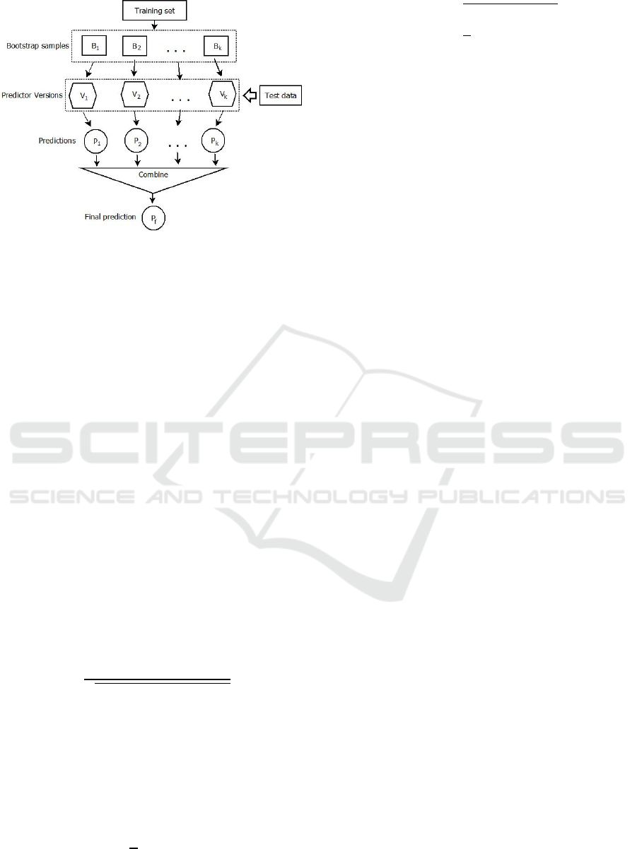
Figure 2: Summary of the process of bagging. From the
training set, k bootstraps are created. Each bootstrap B
1
,
…, B
k
is used to build predictor versions V
1
, …, V
k
which
make separate predictions P
1
, …, P
k
. The final prediction
P
f
is a combination (average for regression, majority
voting for classification) of all the predictions.
2.2.3 Evaluation Criteria
To evaluate the performance of the regression
models, we examine the degree of similarity
between the actual values of the target attribute, and
the predicted values returned by the models. To
assess how well the models will generalize to an
independent dataset, 10-fold cross validation is used
(Kohavi, 1995). The degree of similarity between
the actual and predicted values is checked via three
criteria: the Pearson correlation coefficient, mean
absolute error and root mean squared error.
The Pearson correlation coefficient, R, is a
measure of the linear dependence between X =
{X
1
,…,X
n
} and Z = {Z
1
,…,Z
n
}. It gives a value
between -1 and +1 where -1 stands for total negative
correlation, 0 for no correlation and +1 for total
positive correlation. It can be defined as follows
(Rodgers and Nicewander, 1988):
=
∑
−
−
̅
∑
−
∑
−
̅
(1)
where
and
̅
are means of and respectively.
Mean absolute error (MAE) and root mean
squared error (RMSE) are both widely used in
prediction tasks to measure the amount of deviation
of the predicted values from the actual values. The
two are defined in the following way:
=
1
|
−
|
(2)
=
1
|
−
|
(3)
Where n is the number of predictions,
, …,
are
the actual and
, …,
are the predicted values
respectively (Moore, 2007).
2.3 Classification
The different levels of mRS scores can be viewed as
different categories and hence predicting the mRS
score can be viewed as a multi-class classification
problem. We consider three classifiers in this study.
Two of them are widely used classification
algorithms: logistic regression (McCullagh, 1980)
and C4.5 decision tree (Quinlan, 1993). The choice
of logistic regression is motivated by the fact that it
is the standard classification method used in clinical
trial studies. As for decision tree, it gives a good
diagrammatic representation of the prediction
process as well as proving to be empirically
successful in classification tasks.
The other classification method in this study is
actually one that uses the results of the regression
method involving bagging and model trees. Once a
numeric prediction is obtained from the regression
method, we round it to the nearest integer and assign
the instance to the class corresponding to that
integer. We denote this approach here as
classification via regression.
The evaluation criterion for the classification
algorithms used in this study is accuracy – the
percentage of cases where the actual and the
predicted classes are the same. For the prediction of
mRS-90 score, however, we may consider a
predicted score which is close enough to the actual
score to be fairly accurate as well. We therefore
define “near-accuracy” to be the percentage of cases
where the prediction is either fully correct or is
incorrect by a margin of just one score, and use it as
an additional evaluation metric.
3 RESULTS
3.1 Regression Models to Predict
mRS-90
Supervised regression is performed on the stroke
data to predict the patient outcome after 90 days of
stroke onset. The target attribute is mRS-90, the
mRS score after 90 days, and the predictive
HEALTHINF 2017 - 10th International Conference on Health Informatics
182

attributes are all the other attributes described in
Table 2. We construct an M5 model tree and
compare its results with linear regression, the most
commonly used method for regression analysis. We
then apply bootstrap aggregating (bagging) using
M5 model trees and separately linear regression
models as respective base predictors. For
comparison purposes, we construct also the simple
regression model whose prediction is always the
average of the values of the dependent variable in
the training set.
Parameter optimization is done for both model
tree and bagging. For M5 model trees, we
experiment with the minimum number of instances
to allow in a leaf. It is found that having a minimum
of 10 instances in the leaf produces the best
performing tree. Increasing this number creates
shorter trees that underfit the data while reducing
this number creates larger trees that are prone to
overfitting. For bagging, we experiment with
different number of iterations for bootstrapping
(number of bags) and different bootstrap sizes. Our
conclusion is that 10 iterations with each bootstrap
containing the same number of instances as the
training set produces the best results.
Table 3 compares the results of these five
methods in terms of correlation coefficient (R),
mean absolute error (MAE) and root mean squared
error (RMSE). We can observe from the table that
bagging used in tandem with M5 model trees
performs much better than all the other techniques.
An interesting observation is that M5 model tree
(without bagging) shows an impressive improve-
ment over linear regression in terms of mean
absolute error, but performs only slightly better in
terms of root mean squared error. Large errors have
a relatively greater influence when the errors are
squared. So as the variance associated with the
Table 3: Comparison of different regression methods on
stroke data in terms of R, MAE and RMSE. For R, higher
values indicate better model fit, whereas for the MAE and
RMSE metrics lower values are better.
Method R MAE RMSE
Average Prediction -0.136 1.235 1.461
Linear regression 0.779 0.654 0.916
M5 model tree 0.785 0.577 0.905
Bagging with Linear
Regression
0.783 0.649 0.908
Bagging with M5 model
trees
0.822 0.537 0.832
frequency distribution of the error magnitude
increases, the difference between MAE and RMSE
also increases (Willmott and Matsuura, 2005). It
therefore makes sense that a variance-reducing
procedure like bagging should reduce RMSE when
applied to model trees, as observed in Table 3. Note
also that bagging does not have the same kind of
effect in improving the performance of linear
regression.
To see if the improvement is statistically
significant, we perform paired t-tests in terms of
correlation coefficient on each pair of the four
methods considered. The difference between means
for each pair are examined at a p-value of 0.05. The
results of the tests are presented in Table 4, showing
that the bagging method with M5 model trees
performs significantly better than the other four
methods on the stroke dataset.
Table 4: Results of statistical significance analysis on
correlation coefficient with p-value of 0.05. Each cell
represents the result of the paired t-test between a pair of
algorithms. If the algorithm in the row is significantly
better than the one in the column, a ‘>>’ is shown. If it is
significantly worse, a ‘<<’ is shown. A ‘<->’ indicates that
there is no statistically significant difference.
Avg
Pred
Lin
Reg
M5
tree
Bagging
Lin
Reg
Bagging
M5
trees
Avg Pred
- << << << <<
Lin Reg
>> - <-> <-> <<
M5 tree
>> <-> - <-> <<
Bagging
Lin
Reg
>> <-> <-> - <<
Bagging
M5
trees
>> >> >> >> -
3.1.1 Observations from the M5 Model Tree
We investigate the model returned by the M5 model
tree algorithm to find insights about stroke outcome.
Figure 3 shows the model tree where each leaf is a
linear equation. The equations appear below. The
sign and magnitude of coefficients of each predictive
attribute in the equations give an indication of how
the output attribute responds to changes in the given
input attribute. The continuous variables age and
NIHSS at admission are scaled to the range between
0 and 1, so that the magnitudes of all attributes are
within the [0,1] range.
Predicting Outcome of Ischemic Stroke Patients using Bootstrap Aggregating with M5 Model Trees
183

Figure 3: The M5 model tree built on the stroke dataset
with minimum 10 instances in each leaf. Each leaf is a
linear model predicting the target attribute mRS-90. The
numbers under the leaves indicate how many instances are
covered under that particular linear model.
LM 1 (here the value of mRS at discharge is 0)
mRS 90 days =
- 0.1309 * Subtype - Large Vessel
- 0.1472 * Subtype - Small Vessel
- 0.1552 * Subtype - Cardio
- 0.0532 * Subtype - Crypto
- 0.1454 * Subtype - other
+ 0.064 * NIHSS at admission
+ 0.0189 * MRS before admission
+ 0.0996 * Age
+ 0.0155 * Diabetes
- 0.0472 * Antiplatelets
+ 0.0534 * mRS at discharge
+ 0.1285
LM 2 (here the value of mRS at discharge is 1)
mRS 90 days =
0.0446 * Subtype - Large vessel
- 0.0837 * Subtype - Small vessel
- 0.4857 * Subtype - Cardio
- 0.6028 * Subtype - Crypto
- 0.0827 * Subtype - other
+ 0.3298 * NIHSS at admission
+ 0.084 * MRS before admission
+ 0.4344 * Age
+ 0.0959 * Diabetes
- 0.0137 * Tobacco
+ 0.2618 * Antihypertensives
- 0.0057 * Antiplatelets
+ 0.1265 * mRS at discharge
+ 0.3596
LM 3 (here the value of mRS at discharge is 2 or 3)
mRS 90 days =
0.3911 * Subtype - Large vessel
- 0.0837 * Subtype - Small vessel
- 0.0882 * Subtype - Cardio
- 0.0832 * Subtype - Crypto
- 0.807 * Subtype - other
+ 1.5475 * NIHSS at admission
+ 0.3333 * MRS before admission
+ 1.5486 * Age
+ 0.4281 * Diabetes
- 0.0137 * Tobacco
- 0.0057 * Antiplatelets
+ 0.0951 * mRS at discharge
- 0.3414
LM 4 (here the value of mRS at discharge is 4 or 5)
mRS 90 days =
- 0.0119 * Subtype - Large vessel
- 0.0837 * Subtype - Small vessel
- 0.0882 * Subtype - Cardio
- 0.0832 * Subtype - Crypto
- 0.0827 * Subtype - other
+ 0.1919 * NIHSS at admission
+ 0.0438 * MRS before admission
+ 0.2979 * Age
+ 0.0567 * Diabetes
- 0.0351 * Tobacco
- 0.0057 * Antiplatelets
- 0.4463 * Neurointervention
+ 1.4419 * mRS discharge
- 3.0914
From the model tree of Figure 3, it is clear that mRS
at discharge plays the major role in deciding the
mRS score at 90 days. The tree simply first decides
what the mRS discharge score is, and then builds
linear models to predict mRS-90 for the patients
with that score. By following the decision branches
of the tree, we can see that the linear models LM 1
and LM 2 corresponds to mRS discharge scores of 0
and 1 respectively. Similarly LM 3 is associated
with mRS discharge scores of 2 and 3, and LM 4
with scores of 4 and 5.
Looking at LM 1, we find that the y-intercept is a
very small value and there is no other attribute that
has a large coefficient that could change the
prediction substantially. This means that the
prediction for almost all patients reaching this point
of the tree will be close to 0. At LM 2, since the
mRS discharge score is 1 with a coefficient of
0.1265 and the y-intercept is 0.3596, the baseline
prediction for this leaf (if all other conditions are not
present) is 0.4861. Older age, higher NIHSS at
admission and presence of antihypertensives
contribute towards increasing the mRS-90 score. On
the other hand, cardioembolic and cryptogenic
strokes contribute significantly towards lowering the
mRS-90 score. At LM 3, if the mRS discharge score
is 2, then the baseline prediction is 2*0.0951 –
0.3414 = - 0.1512. If the mRS discharge = 3, it is
3*0.0951 – 0.3414 = - 0.0561. However, there are
some attributes in this model that may have a major
impact on the final prediction, notably age, NIHSS
at admission, diabetes, large vessel stroke subtype
and mRS before admission. Higher values for some
or all of the above attributes will result in increased
HEALTHINF 2017 - 10th International Conference on Health Informatics
184

mRS-90 score. For LM 4, the baseline prediction is
either 2.6762 (for mRS discharge = 4) or 4.1181 (for
mRS discharge = 5). If a patient reaches this leaf, the
output is likely to be quite high, since only
neurointervention has a major effect of lowering the
mRS-90 score.
3.2 Classification Models to Predict
mRS-90
We now consider the mRS-90 attribute as discrete
(i.e., consisting of individual classes 0, 1, …, 5)
instead of a continuous numeric attribute, and
construct classification models to predict this
discrete attribute. We explore two main approaches
to constructing classification models: One is to apply
traditional multi-class classification techniques;
another one is to use regression followed by
classification (i.e., classification via regression). For
this experiment we choose two well-known and
empirically successful classification algorithms,
namely logistic regression and C4.5 decision tree.
For classification via regression we use the bagging
with M5 model tree method discussed in section 3.1,
and convert the predicted mRS-90 numeric value to
a discrete class by rounding this value to the nearest
integer between 0 and 5.
As a first evaluation metric, we use classification
accuracy (the percentage of correct predictions). But
since there are six different classes with subtle
variations between two adjacent mRS scores, we
also consider the case when the classifier makes an
error, but by only one mRS score. We define the
metric “near-accuracy” to refer to the percentage of
cases in which the classifier either makes an
accurate prediction or makes a wrong prediction
which is either one more or one less than the correct
mRS score.
Table 5 shows a comparison of the performance
of classification via regression with those of multi-
class classification using Logistic regression and
C4.5 decision trees. For comparison purposes, we
include also that majority class classifier which
classifies any test instance with the mRS-90 value
that appears most frequently in the training set.
For C4.5 decision trees, the result of the best
model after experimentation with pruning is shown.
The classification via regression method performs
better in terms of both accuracy and near-accuracy.
Table 6 shows the confusion matrix obtained by this
method. Paired t-tests are performed on the
classification accuracy for the three algorithms. The
results, given in Table 7, show that classification via
regression performs significantly better than logistic
regression, but not significantly better than the C4.5
decision tree at a level of p = 0.05.
Table 5: Comparison of logistic regression, C4.5 and
classification via regression (bagging with M5 model
trees) on the stroke dataset in terms of accuracy and near-
accuracy.
Method Accuracy
Near-
accuracy
Majority class 46.9% 64.4%
Logistic Regression 54.2% 83.6%
C4.5 (with pruning) 56.7% 86.8%
Classification via regression 59.7% 90.0%
Table 6: Confusion matrix for the method of supervised
classification via regression using bagging with M5 model
trees. The rows show the actual mRS scores while the
columns show the ones predicted by the model. The
diagonals (in bold) are the correct predictions. The cells
adjacent to the diagonals (in bold and italic) are near-
correct predictions missing the actual score by 1.
Actual
Predicted
0 1 2 3 4 5
0
159
36
11 0 0 0
1
10
40
19
8 0 0
2 2
15
31
14
1 0
3 0 8
19
21
3
0
4 0 3 5
8
10
1
5 0 3 1 2
8
1
Table 7: Results of statistical significance analysis on
classification accuracy with p-value of 0.05. Each cell
represents the result of the paired t-test between a pair of
algorithms. If the algorithm in the row is significantly
better than the one in the column, a ‘>>’ is shown. If it is
significantly worse, a ‘<<’ is shown. A ‘<->’ indicates that
there is no statistically significant difference.
Majority
class
Logistic
Regression
C4.5
tree
Classif via
regression
Majority
class
- << << <<
Logistic
Regression
>> - <-> <<
C4.5 tree
>> <-> - <->
Classif via
regression
>> >> <-> -
Predicting Outcome of Ischemic Stroke Patients using Bootstrap Aggregating with M5 Model Trees
185

4 CONCLUSIONS
This paper has presented the results of predicting the
90-day outcome of stroke patients based on the data
consisting of demographics, medical history and
treatment records of ischemic stroke patients. The
problem of prediction is treated first as the
regression task of predicting the numeric score
according to the modified Rankin Scale which
measures the degree of disability in patients who
have suffered a stroke. A meta-learning approach of
bootstrap aggregating (bagging) using M5 model
trees as the base learner proved to be a very effective
regression technique in this case, significantly
outperforming other more commonly used
regression methods. The same method, after
translation of the target output from numeric to
nominal, performs better as a multi-class
classification scheme than other commonly used
classifiers.
The high performance of the M5 model tree can
be attributed to the fact that the mRS score at 90
days is highly dependent on one of the attributes -
the mRS score at discharge from the hospital.
Therefore, a model predicting mRS-90 would do
well by dividing the input space into a number of
subspaces defined around the value of mRS at
discharge, building a separate specialized model for
each of the subspaces. A model tree does exactly
that. Examination of the M5 model tree that is
constructed on the stroke dataset reveals that the tree
simply directs the prediction task towards different
ranges of values for the mRS score at discharge. A
multivariate linear regression model is then built for
each of the leaves, which are more specialized for
predicting the outcome of those particular patients.
The superior performance of bagging in enhancing
the prediction results can be explained by the
variance in error of the base M5 model trees. By
examining the model tree prediction errors for the
stroke dataset considered, it is found that the
variability of errors is much higher for model trees
than for other regression methods such as logistic
regression. Since bagging is empirically known to
reduce the instability and error variance of its base
learners, it shows good performance for this
particular dataset.
Further examination of the models reveals
interesting insights into how different factors affect
stroke outcome. It is found, rather unsurprisingly,
that patients who have a low mRS score (≤ 1) at
discharge tend to maintain a low mRS score at 90
days as well. However, patients who have some
minor disability (mRS = 1) at discharge tend to have
poorer outcome if they have older age, more severe
initial stroke and hypertension, while patients
suffering from cardioembolic or cryptogenic types
of stroke actually make a better recovery. The
patients who have slight or moderate disability at the
time of discharge (mRS 2 or 3) may end up in a
wide spectrum of outcomes at 90 days based on
several factors; older age, more severe initial stroke,
presence of diabetes, preexisting disability before
stroke and large vessel thrombosis are associated
with poorer outcome. For patients who have fairly
severe disability at the time of discharge (mRS 4 or
5), only neurointervention performed during the
hospital stay has the effect of improving the
recovery rate after discharge and within 90 days of
stroke.
One limitation of the study is the exclusion of the
patients who died within 90 days of stroke. As
mentioned before, this is in line with other work in
the literature (e.g., the Copenhagen Stroke Study
(Nakayama et al., 1994)), but it would be interesting
in future work to extend our approach to include
these patients. We are also limited by a large amount
of missing values in attributes that are not included
in this study but which may have been instrumental
in stroke outcome prediction. In the future we would
like to address these shortcomings to develop better
models for prediction. Another future goal is to
improve the process of classification via regression
by discovering better ways to translate the numeric
predictions to discrete classes.
ACKNOWLEDGEMENTS
The authors would like to thank Theresa Inzerillo
and Preston Mueller of Worcester Polytechnic
Institute for stimulating discussions around the
analysis of stroke data.
REFERENCES
Adams, H. P., Bendixen, B. H., Kappelle, L. J., Biller, J.,
Love, B. B., Gordon, D. L. & Marsh, E. E. 1993.
Classification of subtype of acute ischemic stroke.
Definitions for use in a multicenter clinical trial.
TOAST. Trial of Org 10172 in Acute Stroke
Treatment. Stroke, 24, 35-41.
Aslam, J. A., Popa, R. A. & Rivest, R. L. 2007. On
Estimating the Size and Confidence of a Statistical
Audit. USENIX/ACCURATE Electronic Voting
Technology Workshop, 7, 8.
Banks, J. L. & Marotta, C. A. 2007. Outcomes validity
and reliability of the modified Rankin scale:
HEALTHINF 2017 - 10th International Conference on Health Informatics
186

Implications for stroke clinical trials a literature
review and synthesis. Stroke, 38, 1091-1096.
Breiman, L. 1996. Bagging predictors. Machine learning,
24, 123-140.
Breiman, L., Friedman, J., Stone, C. J. & Olshen, R. A.
1984. Classification and regression trees, CRC press.
Brott, T., Adams, H., Olinger, C. P., Marler, J. R., Barsan,
W. G., Biller, J., Spilker, J., Holleran, R., Eberle, R. &
Hertzberg, V. 1989. Measurements of acute cerebral
infarction: a clinical examination scale. Stroke, 20,
864-870.
Brown, A. W., Therneau, T. M., Schultz, B. A., Niewczyk,
P. M. & Granger, C. V. 2015. Measure of functional
independence dominates discharge outcome prediction
after inpatient rehabilitation for stroke. Stroke, 46,
1038-1044.
Etemad-Shahidi, A. & Mahjoobi, J. 2009. Comparison
between M5′ model tree and neural networks for
prediction of significant wave height in Lake Superior.
Ocean Engineering, 36, 1175-1181.
Gialanella, B., Santoro, R. & Ferlucci, C. 2013. Predicting
outcome after stroke: the role of basic activities of
daily living predicting outcome after stroke. European
journal of physical and rehabilitation medicine, 49,
629-637.
Hall, M., Frank, E., Holmes, G., Pfahringer, B.,
Reutemann, P. & Witten, I. H. 2009. The WEKA data
mining software: an update. ACM SIGKDD
explorations newsletter, 11, 10-18.
Henninger, N., Lin, E., Baker, S. P., Wakhloo, A. K.,
Takhtani, D. & Moonis, M. 2012. Leukoaraiosis
predicts poor 90-day outcome after acute large
cerebral artery occlusion. Cerebrovascular Diseases,
33, 525-531.
Keith, R., Granger, C., Hamilton, B. & Sherwin, F. 1987.
The functional independence measure. Adv Clin
Rehabil, 1, 6-18.
Kohavi, R. 1995. A study of cross-validation and
bootstrap for accuracy estimation and model selection.
IJCAI.
Marini, C., De Santis, F., Sacco, S., Russo, T., Olivieri, L.,
Totaro, R. & Carolei, A. 2005. Contribution of atrial
fibrillation to incidence and outcome of ischemic
stroke results from a population-based study. Stroke,
36, 1115-1119.
McCullagh, P. 1980. Regression models for ordinal data.
Journal of the royal statistical society. Series B
(Methodological), 109-142.
Moonis, M., Kane, K., Schwiderski, U., Sandage, B. W. &
Fisher, M. 2005. HMG-CoA reductase inhibitors
improve acute ischemic stroke outcome. Stroke, 36,
1298-1300.
Moore, D. S. 2007. The basic practice of statistics, New
York, WH Freeman
Mozaffarian, D., Benjamin, E. J., Go, A. S., Arnett, D. K.,
Blaha, M. J., Cushman, M., Das, S. R., de Ferranti, S.,
Després, J.-P. & Fullerton, H. J. 2016. Heart Disease
and Stroke Statistics-2016 Update: A Report From the
American Heart Association. Circulation, 133, 447.
Nakayama, H., Jørgensen, H., Raaschou, H. & Olsen, T.
1994. The influence of age on stroke outcome. The
Copenhagen Stroke Study. Stroke, 25, 808-813.
Nogueira, R. G., Liebeskind, D. S., Sung, G., Duckwiler,
G., Smith, W. S. & Multi MERCI Writing Committee
2009. Predictors of good clinical outcomes, mortality,
and successful revascularization in patients with acute
ischemic stroke undergoing thrombectomy pooled
analysis of the Mechanical Embolus Removal in
Cerebral Ischemia (MERCI) and Multi MERCI Trials.
Stroke, 40, 3777-3783.
Quinlan, J. R. 1992. Learning with continuous classes. 5th
Australian joint conference on artificial intelligence.
Singapore.
Quinlan, J. R. 1993. C4. 5 Programs for Machine
Learning, San Francisco, Morgan Kauffmann.
Raffeld, M. R., Debette, S. & Woo, D. 2016. International
Stroke Genetics Consortium Update. Stroke, 47, 1144-
1145.
Rankin, J. 1957. Cerebral vascular accidents in patients
over the age of 60. II. Prognosis. Scottish medical
journal, 2, 200.
Rodgers, J. L. & Nicewander, W. A. 1988. Thirteen ways
to look at the correlation coefficient. The American
Statistician, 42, 59-66.
Tan, P.-N., Steinbach, M. & Kumar, V. 2005. Introduction
to data mining, Boston, Addison-Wesley.
Van Swieten, J., Koudstaal, P., Visser, M., Schouten, H. &
Van Gijn, J. 1988. Interobserver agreement for the
assessment of handicap in stroke patients. Stroke, 19,
604-607.
Wang, Y. & Witten, I. H. 1996. Induction of model trees
for predicting continuous classes. European
Conference on Machine Learning. University of
Economics, Prague.
Willmott, C. J. & Matsuura, K. 2005. Advantages of the
mean absolute error (MAE) over the root mean square
error (RMSE) in assessing average model
performance. Climate research, 30, 79-82.
Yong, M. & Kaste, M. 2008. Dynamic of hyperglycemia
as a predictor of stroke outcome in the ECASS-II trial.
Stroke, 39, 2749-2755.
Predicting Outcome of Ischemic Stroke Patients using Bootstrap Aggregating with M5 Model Trees
187
