
Appliance Usage Prediction for the Smart Home with an Application to
Energy Demand Side Management
And Why Accuracy is not a Good Performance Metric for this Problem
Marc Wenninger
1
, Jochen Schmidt
1
and Toni Goeller
2
1
Department of Computer Science, Rosenheim University of Applied Sciences, Rosenheim, Germany
2
MINcom GmbH, Rosenheim, Germany
Keywords:
Real Time Pricing (RTP), Household Appliance Usage Prediction, Demand Side Management.
Abstract:
Shifting energy peak load is a subject that plays a huge role in the currently changing energy market, where
renewable energy sources no longer produce the exact amount of energy demanded. Matching demand to supply
requires behavior changes on the customer side, which can be achieved by incentives such as Real-Time-Pricing
(RTP). Various studies show that such incentives cannot be utilized without a complexity reduction, e. g., by
smart home automation systems that inform the customer about possible savings or automatically schedule
appliances to off-peak load phases. We propose a probabilistic appliance usage prediction based on historical
energy data that can be used to identify the times of day where an appliance will be used and therefore make
load shift recommendations that suite the customer’s usage profile.
A huge issue is how to provide a valid performance evaluation for this particular problem. We will argue why
the commonly used accuracy metric is not suitable, and suggest to use other metrics like the area under the
Receiver Operating Characteristic (ROC) curve, Matthews Correlation Coefficient (MCC) or
F
1
-Score instead.
1 INTRODUCTION
With renewable energy sources, electric grid operators
face a variety of new challenges. One being the highly
variable amount of power produced, e. g. by wind tur-
bines or photovoltaic systems. In order to guarantee
the stability of the grid, the amount of energy in the
grid has to be just right. Hence, supply and demand
must match. Up to now, unexpected power fluctuations
emerged on the demand side only (in particular indus-
trial plants and private households), which could be
balanced for example by gas engines. A wind turbine,
however, generates energy in windy weather condi-
tions, but not necessarily when the power is required
on the demand side. In windless phases (or cloudy
ones in terms of photovoltaic systems), the result is an
undersupply of power in the grid. As power cannot be
stored very efficiently, over-production is also a major
problem for grid operators. Therefore, the problem to
be solved is to balance demand and supply. One step
in this direction is the smoothing of load peaks through
load shifting, i. e., shifting parts of power consumption
to other time periods, in which less power is used.
Our aim is to develop solutions for optimal load
shifting for private consumers using artificial intelli-
gence, and Real-Time-Pricing (RTP) as an incentive
to integrate the customer into the balancing of supply
and demand (see (Hassan et al., 2016) for a discussion
of methodologies to assist grid operators in designing
incentives for consumer participation in demand re-
sponse management taking into account inconvenience
for participating users). RTP are tariffs, in which elec-
tricity cost varies over time (e. g., the price changes
every 15 min) (S.a., 2005a). Studies suggest that RTP
models require a complexity reduction in order to be
accepted by the end-user (S.a., 2005b), as well as that
customers will respond with shaving instead of shifting
of their peak demand (Schleich and Klobasa, 2013).
We therefore combine such tariffs with the knowledge
of a household’s typical power consumption, which
form the basis for an intelligent demand side manage-
ment system. The system is then capable of shifting
loads to better suited time periods through measures
specifically tailored to user behavior. Simulations have
already shown that such systems can effectively re-
duce the peak-to-average ratio (Mohsenian-Rad and
Leon-Garcia, 2010). We aim to reduce the system’s
complexity sufficiently, in order to enable technically
unversed persons to make use of it as well.
Smart meters are used for metering and billing;
Wenninger, M., Schmidt, J. and Goeller, T.
Appliance Usage Prediction for the Smart Home with an Application to Energy Demand Side Management - And Why Accuracy is not a Good Performance Metric for this Problem.
DOI: 10.5220/0006264401430150
In Proceedings of the 6th International Conference on Smart Cities and Green ICT Systems (SMARTGREENS 2017), pages 143-150
ISBN: 978-989-758-241-7
Copyright © 2017 by SCITEPRESS – Science and Technology Publications, Lda. All rights reserved
143

Tariff Server
Billing Component
Actuator / Switch
Information System
Home Automation
Billing System
Headend System
Smart-Meter
Smart-Meter Infrastructure
Customer
Provider
Gateway
Real-Time-Pricing
Tariffs
Figure 1: The big picture: the system for transmission and
evaluation of tariff information is decoupled from the smart
meter infrastructure. The customer has full control over the
home automation gateway, therefore no privacy issues arise.
This article’s focus is on exploiting RTP tariffs on the home
automation side using AI methods.
these devices are digital electricity meters that connect
to the utility company over a communication network.
The design of a system for residential smart grid appli-
cations is discussed, e. g., in (Viswanath et al., 2016).
As shown in Fig. 1, the system being developed in
our project for transmission and evaluation of tariff
information is decoupled from the smart meter infras-
tructure. The evaluation of tariffs in the home automa-
tion gateway may be augmented by a large variety of
additional information, for example: historical energy
consumption data of single appliances or the entire
household; the presence or absence of residents; or
weather forecasts. With this data, using artificial in-
telligence methods, behavior patterns can be detected;
combined with tariff information the optimal use of
household appliances can be computed. Based on the
results of these computations, appliances can be con-
trolled directly using the home automation system. A
main challenge is to avert that power cost minimization
has negative consequences for the user. This requires
appliance usage profiling.
Appliance usage profiling and prediction is al-
ready discussed in various publications, where, e. g.,
ON/OFF probabilities are used to build a non-
homogeneous Markov Chain to model end-use energy
profiles on appliance level (Kang et al., 2014); (Chang
et al., 2013) propose a daily pattern based probability
model. Decision trees and Bayesian network-based
prediction are utilized in (Arghira et al., 2012) to dis-
cover behavior patterns within sequential data; (Heier-
man and Cook, 2003) propose using the ED (Episode
Discovery) data-mining algorithm for this purpose.
(Hawarah et al., 2010) predict the user behavior with
bayesian networks and (Basu et al., 2013) compare the
performance of different classifiers such as bayesian
networks, decision trees and decision tables for predict-
ing the future 24h power consumption of an appliance.
In this paper, as a first step, we present an approach
for predicting appliance usage (e. g., for dishwashers,
washing machines etc.), which allows the automation
system to either control the appliances directly, or to
give recommendations to the residents in which time
period using the appliance would result in lower energy
costs, based on the users’ normal behavior patterns,
which are learned from historical data automatically.
This requires some kind of energy load prediction.
Our prediction model is based on the appliance’s us-
age cycles, thus requiring the extraction of appliance
operation cycles (start/end time) from its electricity
metering data (Stephen et al., 2014).
2 PREDICTION METHOD
Probabilistic Model.
There are basically two main
factors that need to be taken into account when com-
puting the probability that an appliance will be used:
The time elapsed since it was used last and the time
of day it is usually used. For example, a dishwasher
will typically be switched on in more or less regular
intervals and only at certain times of day (e. g., nor-
mally not at 2 a. m.). We model these separately as
probability distribution functions (PDFs), where in the
following
E
will denote the event elapsed time and
D
the event time of day. To give recommendations to the
user, the combined probability of these two events has
to be calculated and must be above a defined threshold
to initiate a recommendation:
P(E ∩ D) = P(E | D)P(D)
if independent
= P(E)P(D) .
(1)
Statistical independence of
E
and
D
is assumed here;
although strictly speaking not necessary, as the condi-
tional probability
P(E | D)
can be computed from the
data if a sufficient amount of representative data are
available. As this is quite often not the case (cf. Sect. 4
for details on typical data sets), the independence as-
sumption results in more stable estimates of
P(E ∩ D)
.
That independence is valid can be checked on the data
set by computing the product on the right and middle
of (1), and checking that equality holds.
The probability
P(E)
that the appliance is not used
for a time period
t
(here measured in minutes) is mod-
eled by an exponential distribution:
P(E) = P(E ≤ t) =
(
1 − e
−λt
t ≥ 0
0 t < 0
. (2)
A maximum likelihood estimate of the parameter
λ
can be obtained from a sufficiently large data set by
SMARTGREENS 2017 - 6th International Conference on Smart Cities and Green ICT Systems
144
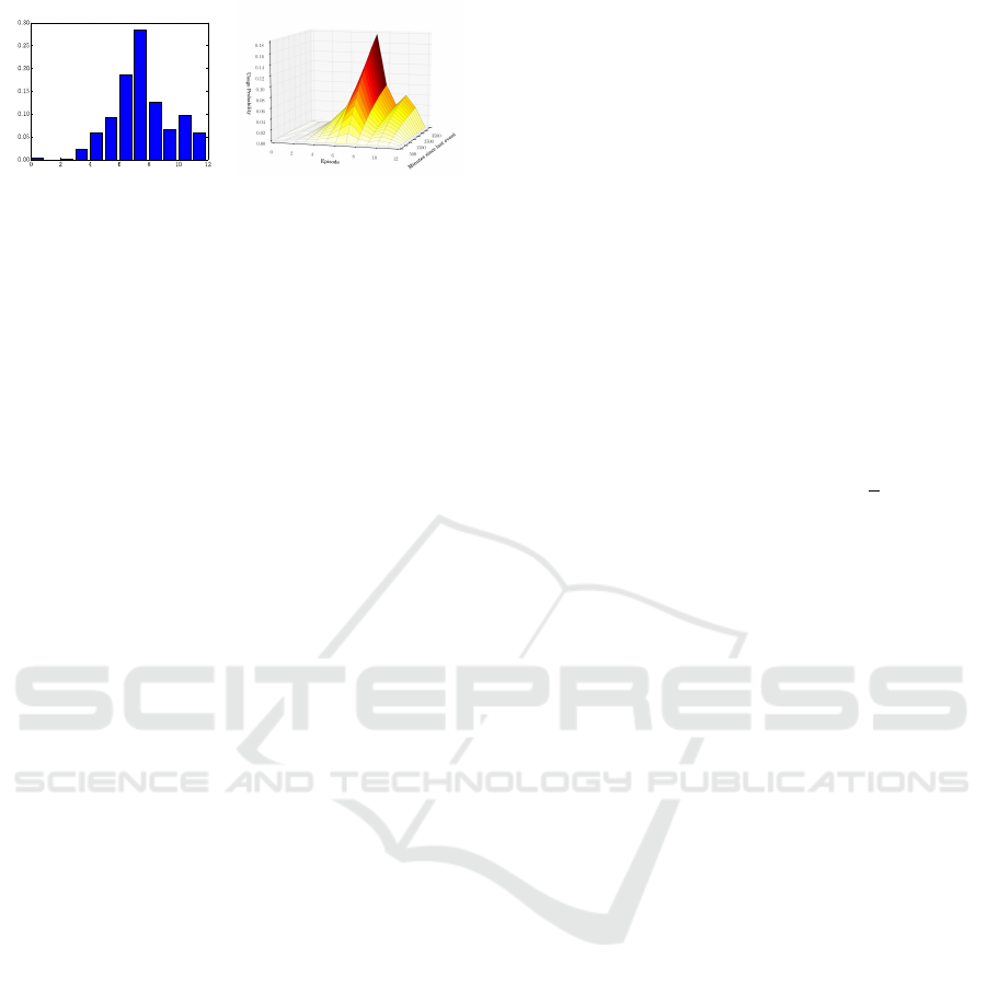
Figure 2: Example of estimates for
P(D)
(discrete density of
appliance usage throughout the day, left) and the combined
cumulative distribution
P(E ∩ D)
(right). Episode length is
2h, resulting in 12 episodes per day.
computing the mean value of the time periods between
consecutive appliance-switch-on events. A good es-
timate of
λ
will be obtained when the time between
usage is fairly regular, resulting in a small value for
the variance of the time periods.
In contrast to using a continuous distribution for
E
, a discrete PDF for the event
D
is estimated from
the sample data by computing relative frequencies of
appliance usage viewed over the 24 hour time period
of a day. This period has to be divided into discrete
intervals, which we will call episodes in the follow-
ing. An episode must be sufficiently large, so that
statistically valid relative frequencies (which are an
estimate of the probability that the appliance is used
in a particular episode) can be obtained. On the other
hand, it has to be small enough to be of practical use.
We found episodes having a length of 1h to 2h to be
a good compromise. To avoid issues with episodes
where no samples are contained in the data set, leading
to density values of zero, the Parzen window approach
(Parzen, 1962; Duda et al., 2000) can be applied, which
is basically an interpolation and smoothing method,
typically using Gaussians. Figure 2 shows an example
of a discrete PDF computed from the GREEND data
set (Monacchi et al., 2014).
Inactivity Detection.
Most household appliances
with non-homogeneous distribution in electricity con-
sumption require the user’s presence when starting
the appliance. Thus, the prediction of a household
appliance usage is often accompanied by a prediction
of the home’s occupancy; in some cases an appliance
might even be directly linked to the presence of a spe-
cific person. Without ground truth on the occupancy,
a strong indication that can be found in the historical
electricity data is the usage of such appliances in the
recent history. We therefore add knowledge of the
events that occurred in recent history to the prediction
by lowering the probability in case no appliance was
used in recent episodes. We found that the past 12h to
24h are of specific interest and improve the prediction
significantly. This approach may be replaced by more
sophisticated occupancy detection algorithms, which
are not the focus of this paper.
Threshold Estimation.
Now that the usage proba-
bility can be computed at any time of day, a threshold
has to be set that determines whether the home au-
tomation system turns on the appliance (or gives a
recommendation to the user to do so). Note, that the
absolute values of
P(E ∩ D)
depend heavily on the
time interval chosen as episode duration. Obviously,
longer episodes result in higher probabilities for appli-
ance usage during this period; e. g., using 2h instead of
1h episodes would approximately double the probabil-
ities (exactly for uniform distribution, less so for uni-
/multi-modal densities). We propose to compute the
threshold automatically from the training data by cal-
culating
P(E ∩ D)
for each episode of the training set.
Let
p
i
be the predicted probability at the
i
-th turn-on
event of a total of
N
that occurs in the data, the thresh-
old
θ
p
is computed as the mean:
θ
p
=
1
N
∑
N−1
i=0
p
i
. If
extreme outliers are expected or more control over the
threshold is desired, the Median or any other quantile
may be used instead.
Extended Model.
The model described above
works well when appliances are typically used in fairly
regular intervals, like dishwashers. There are scenar-
ios, however, where it fails; e. g., a household may
use the washing machine every Saturday, but not only
for a single washing cycle but two or three times in a
row. While the estimate for
P(D)
will still be valid,
the parameter
λ
of the exponential distribution will be
invalid. This issue can be overcome by introducing an
additional discrete random variable
U
, describing how
many times an appliance has been used during the past
n
e
episodes. The parameter
n
e
can be adjusted to the
appliance at hand; e. g., for a washing machine a 10h
period may suffice. Generalization of (1) gives:
P(E ∩ D) =
∞
∑
i=0
P(E ∩ D | U = i)P(U = i)
=
n
m
∑
i=0
P(E ∩ D | U = i)P(U = i)+
P(E ∩ D | U > n
m
)P(U > n
m
) ,
(3)
where
n
m
is an upper limit for the number of times an
appliance is used that can be derived from the training
data (a washing machine may be switched on 3 or
4 times in a 10h interval, but not 20 times); from a
certain value of
i
onwards, all probabilities
P(U = i)
will usually be zero.
Appliance Usage Prediction for the Smart Home with an Application to Energy Demand Side Management - And Why Accuracy is not a
Good Performance Metric for this Problem
145

3 ACCURACY IS NOT A GOOD
PERFORMANCE METRIC
In many publications on appliance usage prediction or
energy load disaggregation the performance metric ac-
curacy is chosen to evaluate the proposed classification
methods. The accuracy
A
is defined as the proportion
of data that has been classified correctly:
A =
T
P
+ T
N
n
, (4)
where
n
is the total number of events,
T
P
is the num-
ber of positive events and
T
N
is the number of nega-
tive events that have been classified correctly (True
Positives and True Negatives, respectively). For the
problem at hand we get a true positive if the algorithm
predicts that an appliance is running during a given
time period and the appliance is actually doing so. In
the same manner, for a true negative the prediction is
that the appliance is off and this is truly the case. The
denominator n is then the total number of episodes.
The main issue with this commonly chosen metric
is that it is not meaningful for rare events; this is known
as the accuracy paradox (Zhu and Davidson, 2007;
Valverde-Albacete and Peláez-Moreno, 2014). Rare
events, however, are in most
1
cases the standard when
looking at the problem of appliance usage prediction!
Consider, for instance, a dishwasher: this appliance
is normally used quite regularly, say every other day,
where it takes about 2h to finish its cycle. This means,
though, that in 96% of the total time the dishwasher is
off. Even if it is used twice as often, i. e., every day, it
will still be off 92% of the time. Publications making
use of accuracy, such as (Heierman and Cook, 2003;
Barbato et al., 2011; Basu et al., 2013; Lee et al., 2013;
Lachut et al., 2014), could therefore easily be outper-
formed for rare events by simply always predicting no
occurrence (i. e., a Negative), which will result in an
accuracy of 96% for the dishwasher example above.
The issue of selecting an appropriate metric has
been addressed before by several authors from vari-
ous fields (Cook, 2007; Hand, 2009; Powers, 2011;
Makonin and Popowich, 2015). The overall perfor-
mance of a binary classifier is usually captured using
the Receiver Operating Characteristic (ROC), which
is a plot of the true positive rate (TPR, also called sen-
sitivity, recall, or detection rate) vs. false positive rate
(FPR). These are given by:
TPR =
T
P
P
, FPR =
F
P
N
, (5)
where
F
P
is the number of negative events that have
been classified incorrectly as positive ones,
P
is the
1
The possible exception being appliances like fridges or
freezers.
total number of positive and
N
the total number of
negative events, with
n = P + N
. Examples of ROC
plots are shown in the experiments section in Fig. 4.
A perfect classifier would show a rectangular curve,
while the main diagonal indicates complete random-
ness. Any point on the curve can be selected for classi-
fication by choosing the classifier’s parameters appro-
priately. Every point results in a different value for the
accuracy
A
calculated as shown in
(4)
. In publications,
where only accuracy is presented, this will usually be
the point on the ROC curve where the maximum value
is obtained.
This is similar for the following two metrics, the
F
1
-Score and the Matthews Correlation Coefficient
(MCC):
F
1
= 2 ·
PREC · TPR
PREC + TPR
, PREC =
T
P
T
P
+ F
P
, (6)
where
PREC
is called precision, and
TPR
is the true
positive rate (recall) from (5).
MCC =
T
P
T
N
− F
P
F
N
p
PN(T
P
+ F
P
)(F
N
+ T
N
)
, (7)
with
F
N
and
T
N
being the number of false and true
negatives, respectively.
F
1
ranges from
0
to
1
, the
MCC, being a correlation coefficient, ranges from
−1
to
+1
. In both cases zero indicates total randomness
and one perfect classification. While the
F
1
-Score also
suffers from a bias when sample sizes for positive and
negative data are different, the MCC balances these. It
is therefore much better suited for measuring classifier
performance in cases, where events are rare.
In contrast to all these metrics, which measure per-
formance for a single point on the ROC curve, the Area
Under Curve (AUC) tries to capture the quality of the
whole ROC in single numerical value by computing
the area under the ROC:
AUC =
Z
1
0
ROC dFPR. (8)
For a correctly evaluated classifier, the AUC will range
from
0.5
(total randomness) to
1
(perfect). Although
reducing two dimensions to a single one without los-
ing information is not feasible, AUC is still a valid
metric for overall performance, and much better suited
than accuracy. Extensions of AUC can be found in
literature, e. g. (Hand, 2009), who suggests a weighted
AUC.
Unfortunately, knowledge regarding evaluation
metrics does not seem to be widely spread in the en-
ergy usage prediction and disaggregation community.
This has been criticized before by several authors like
(Kim et al., 2011; Makonin and Popowich, 2015), alas
with apparently little effect. We propose using AUC,
F
1
, and MCC, and will give results for all three metrics
in this paper’s experiments section.
SMARTGREENS 2017 - 6th International Conference on Smart Cities and Green ICT Systems
146

4 EXPERIMENTAL RESULTS
Evaluating the proposed prediction method requires
high resolution power consumption measurements of
individual appliances. A few publicly available data
sets already exists, usually containing the whole house
and appliance level energy consumption data (see Ta-
ble 1). We selected homes from the GREEND data
set (Monacchi et al., 2014) to evaluate our prediction
model. This set was chosen as it provides enough mea-
surements to enable statistical analysis of events and
is of sufficient data quality. Other data sets, such as
REDD (Kolter and Johnson, 2011) or ECO (Beckel
et al., 2014), do not provide enough data or the re-
quired quality (e. g., there are often long periods where
data is missing). The GREEND data set provides mea-
surements of eight homes with a varying amount of
appliances and measuring periods ranging from 134 to
500 days. The data are sampled with a rate of 1 Hz and
provide the power consumption in Watts per appliance.
Comparing our results to previous usage prediction
publications proved to be infeasible as the results are
not comparable due to the chosen data set or evaluation
metric. Evaluations using artificially generated data
(Heierman and Cook, 2003; Barbato et al., 2011) are
not comparable as the amount of introduced random-
ness will dictate the result, especially for rare events
such as dishwasher usage. We do not consider these
evaluations as valid. Publications evaluating appli-
ance usage prediction on short data sets, e. g. REDD
(Truong et al., 2013a; Truong et al., 2013b), are also
not comparable due to the insufficient amount of data
in the set. REDD contains data for only up to 19 days,
a duration that we consider totally inadequate for train-
ing and evaluation of rare events such as dishwasher
usage.
Extracting Events.
As the prediction is based on
event occurrences, where an event is defined by the
start and end of an appliance’s usage cycle, in a first
pre-processing step the events must be extracted from
the continuous power consumption data stream. As the
start and end of an event are not provided by any of the
data sets listed in Table 1, the performance of the event
extraction cannot be measured against ground truth.
We first aggregate the data to
1/60
Hz by averaging
the power consumption. The start and stop of an event
are defined by the rising and falling edge of the signal,
which allows using a threshold method. In case an
appliance’s power consumption falls below the thresh-
old during an event, this event will be partitioned, thus
(incorrectly) generating multiple usage cycles instead
of a single one. For the method proposed in this paper,
the partitioning will not be an issue for computing the
discrete estimate of
P(D)
in
(1)
; however, the estimate
of
λ
of the exponential distribution
P(E)
in
(2)
would
be distorted. We overcome this problem by defining an
individual threshold for each type of appliance, which
minimizes the partitioning, and then only use events of
sufficient length. Table 2 gives a statistical overview
of the extracted events for appliances selected from
the GREEND data set.
Results.
The extracted events were split into two
disjoint parts,
60%
for training and
40%
for evalu-
ation. The training set is used to estimate
λ
in
(2)
by calculating the mean value between consecutive
appliance-switch-on events. As an example,
λ
for the
dishwasher in house 3 is 2274 minutes (
≈ 1.6
days).
An episode length of 360 minutes was chosen, which
divides the day into four partitions. A smaller episode
length leads to a more time precise prediction task, and
vice versa. As we do not require high time precision,
but rather a recommendation window that suites the
user’s behavior patterns, four partitions per day give a
reasonable recommendation window.
The probability
P(D)
from
(1)
for each episode is
calculated by binning the appliance-switch-on event
duration into the corresponding episode-bin. Figure 3
shows
P(E ∩ D)
for the dishwasher in house 3. It
clearly shows the characteristics of
P(D)
: The appli-
ance is not likely to be used in the morning, very likely
during midday and medium in the evening. With this
information we can define the user’s preferred usage
window and only recommend load shifts within this
window. It also shows the effect of
P(E)
on the com-
bined probability, as the probability drops immediately
after the appliance is switched on. This respects the
mean duration between events, hence no load shift rec-
ommendation must be made until a significant proba-
bility is reached in the successive episodes.
For usage prediction performance comparison be-
tween the appliances in different homes we calculate
the ROC and the area under the ROC curve (AUC) by
changing the threshold probability at which the predic-
tion will consider the appliances as being used; also
the
F
1
-Score and MCC. The results are highly depen-
dent on the house and appliance (cf. Table 2) The worst
prediction result is obtained for the fridge in house 1,
a MCC of 0.029, which is complete randomness. The
reason is insufficient data: Table 2 shows that there
were only 15 events available in the whole data set,
therefore good performance cannot be expected.
Although very good results can typically be
achieved for fridges, these are not ideal for load shift-
ing; dishwashers, washing machines and dryers on
the other hand are of special interest, as they are well
suited for this purpose. ROC curves for these appli-
Appliance Usage Prediction for the Smart Home with an Application to Energy Demand Side Management - And Why Accuracy is not a
Good Performance Metric for this Problem
147
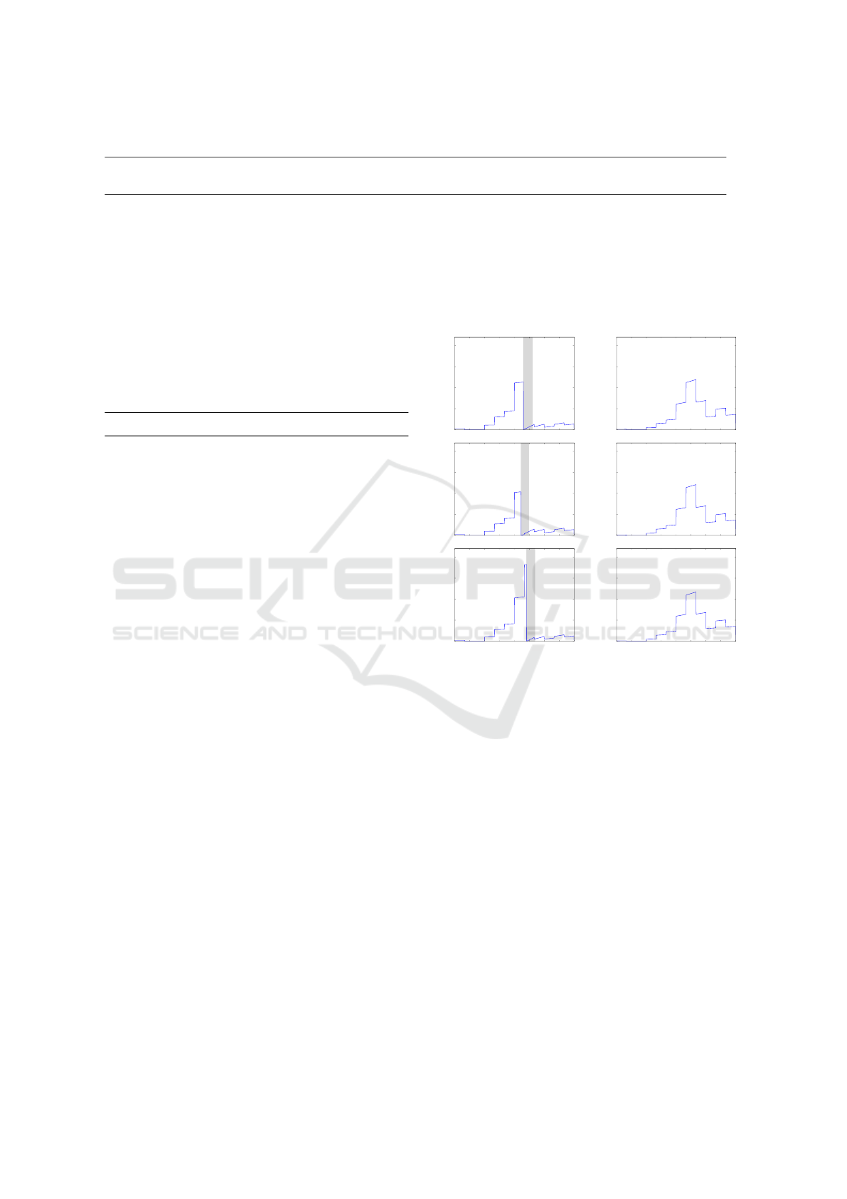
Table 1: Publicly available appliance and whole house energy consumption data sets.
Data set Reference Location
Duration/
house
# of
houses
Appliance
sample intvl
Aggregate
sample intvl
REDD (Kolter and Johnson, 2011) MA, USA 3–19 days 6 3 sec 1 sec & 15 kHz
Smart* (Barker et al., 2012) MA, USA 3 months 3 1 sec 1 sec
AMPds 2 (Makonin et al., 2016) BC, Canada 2 years 1 1 min 1 min
UK-DALE
(Kelly and Knottenbelt, 2015)
London, UK 3–26 months 5 6 sec 1–6 sec & 16 kHz
ECO (Beckel et al., 2014) Switzerland 8 months 6 1 sec 1 sec
GREEND (Monacchi et al., 2014) Italy & Austria 12 months 9 1 sec –
Dataport (Pecan Street Inc., 2014) TX, USA 0–2.75 years 824 1 min 1 min
DRED (Uttama Nambi et al., 2015) Netherlands 2 months 1 1 sec 1 sec
Table 2: Statistics of extracted events of the GREEND data
set, providing the days between first and last events as well
as the total events count for six different homes. Also shown
are resulting performance metrics using an episode length of
360 minutes.
H# Appliance Days Events AUC F
F
F
1
1
1
MCC
0 coffee maker 308 676 0.703 0.708 0.498
0 dishwasher 306 143 0.684 0.389 0.348
0 fridge freezer 309 7353 0.999 0.999 0.972
0 lamp 307 215 0.701 0.524 0.344
0 television 117 445 0.567 0.852 0.251
0 washing mach. 309 256 0.591 0.378 0.190
1 bedside light 473 456 0.859 0.704 0.580
1 dishwasher 472 248 0.651 0.335 0.213
1 dryer 473 405 0.859 0.811 0.763
1 fridge 454 15 0.550 0.017 0.029
1 washing mach. 467 166 0.839 0.415 0.390
2 coffee maker 494 512 0.580 0.333 0.180
2 dishwasher 495 477 0.856 0.654 0.553
2 dryer 495 424 0.828 0.596 0.499
2 television 497 1446 0.770 0.786 0.618
2 washing mach. 497 794 0.809 0.728 0.634
3 coffee maker 456 250 0.719 0.397 0.349
3 dishwasher 456 211 0.843 0.414 0.394
3 fridge 460 1100 0.917 0.909 0.818
3 television 461 849 0.827 0.783 0.652
3 washing mach. 457 279 0.789 0.392 0.329
4 fridge freezer 282 137 0.802 0.471 0.451
4 television 280 2242 0.753 0.675 0.543
4 television 2 280 1657 0.657 0.706 0.332
4 washing mach. 263 81 0.641 0.198 0.168
5 fridge freezer 418 13054 0.734 0.985 0.665
5 lamp 416 322 0.627 0.420 0.193
5 television 417 1297 0.867 0.880 0.710
5 television 2 417 677 0.582 0.561 0.247
5 washing mach. 415 521 0.624 0.396 0.229
ances are shown in Fig. 4. The best prediction results
for this type of appliance were achieved for the dryer
in house 1 with an AUC of 0.859 and MCC of 0.763.
The home with the most predictable dishwasher and
washing machine usage is house 2, with AUC 0.856,
MCC 0.553 (dishwasher), and AUC 0.809, MCC 0.634
(washing machine). On the other hand, the results for
house 0 are AUC 0.684, MCC 0.348 (dishwasher) and
AUC 0.591, MCC 0.190 (washing machine). The rea-
0 0 0 3 06 09 12 15 18 2 1 0 0
0.00
0.05
0.10
0.15
0.20
0 0 0 3 06 09 12 15 18 2 1 0 0
0.00
0.05
0.10
0.15
0.20
0 0 0 3 06 09 12 15 18 2 1 0 0
0.00
0.05
0.10
0.15
0.20
0 0 0 3 06 09 12 15 18 2 1 0 0
0.00
0.05
0.10
0.15
0.20
0 0 0 3 06 09 12 15 18 2 1 0 0
0.00
0.05
0.10
0.15
0.20
0 0 0 3 06 09 12 15 18 2 1 0 0
0.00
0.05
0.10
0.15
0.20
Figure 3: Usage probability prediction and real occurrence
for each day of a dishwasher during 2015/2/1 to 2015/2/6
(l.r.t.b). The gray area marks the time the appliance is
switched on, the curve the probability of the device being
switched on at each minute. For a clearer demonstration, we
chose an episode length of 120 minutes; the x-axis is labeled
by the hour of the day.
son for the performance difference compared to other
homes lies in behavior changes of the inhabitants of
house 0, which can be shown by comparing the proba-
bility distribution
P(D)
for training and evaluation data
(see Fig. 5). While in the dishwasher’s training data
the first episode of a day has a probability of 0.37, in
the evaluation data it is 0.08. The probability densities
show that the events where moved to the last episode
of the day, an episode with a low probability in the
training data. The changes, represented as the mean
square error (MSE), between training and evaluation
are 0.0462 for house 0 and 0.0033 for house 2. Thus,
the preconditioned behavior consistency is no longer
given in house 0, a problem which could be overcome
by analyzing recent behavior changes and adapting
P(D) accordingly. This is a topic for future research.
SMARTGREENS 2017 - 6th International Conference on Smart Cities and Green ICT Systems
148
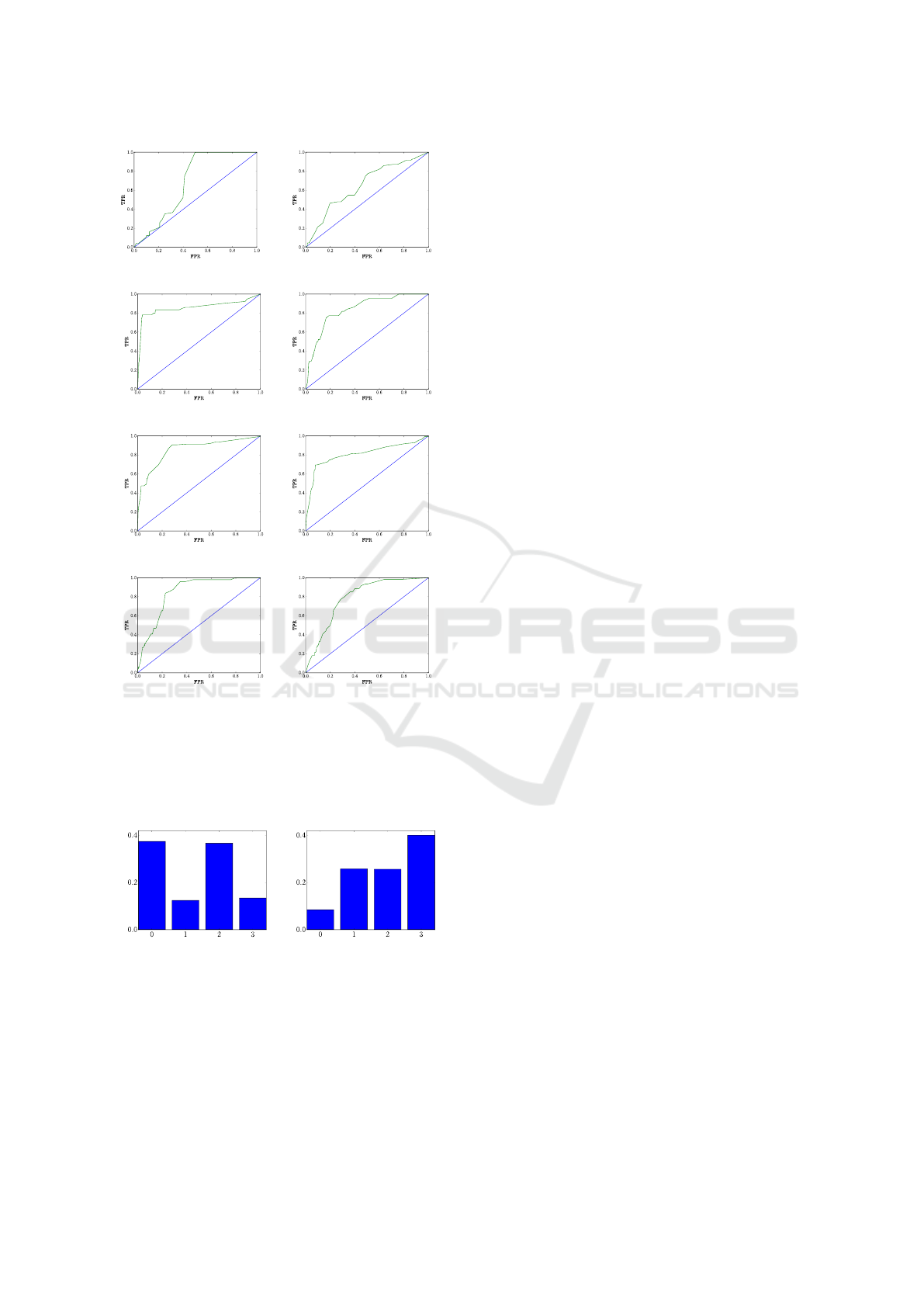
(a) H#0 – dishwasher (b) H#1 – dishwasher
(c) H#1 – dryer (d) H#1 – washing machine
(e) H#2 – dishwasher (f) H#2 – washing machine
(g) H#3 – dishwasher (h) H#3 – washing machine
Figure 4: Examples of ROC curves of the prediction al-
gorithm on the GREEND data set. Dishwasher, washing
machine, and dryer were selected as these appliances are par-
ticularly suited for load shifting. A perfect classifier would
show a rectangular curve, while the main diagonal indicates
complete randomness.
(a) training data (b) test data
Figure 5:
P(D)
of the dishwasher in house 0 shows signifi-
cant difference between (a) training and (b) evaluation.
5 CONCLUSION
We presented probabilistic models for appliance usage
prediction based on historical energy data. The appli-
cation we have in mind is to give recommendations to
the user (or home automation system), whether switch-
ing an appliance on would result in lower energy costs
whilst taking into account the appliance’s typical us-
age pattern in the particular household. An important
topic for future work is to investigate how to handle
long term behavior changes like those found in house
0 of the GREEND data set for the dishwasher, and
how to adapt the model over time. The results on the
GREEND data set look promising; there are currently
no publications available providing results for this kind
of application that we could use as a benchmark, as the
evaluation method is often invalid due to the accuracy
paradox, or the amount of data used for training is
insufficiently low to provide reliable results. At the
moment, it is not yet clear what the best and most
meaningful performance evaluation metric for this sort
of prediction problem would be, as in contrast to usual
classification problems, the goal is not to predict the
exact time an appliance is used, but rather give a rec-
ommendation at convenient times. We presented our
results using the AUC,
F
1
and MCC metrics to provide
a comparable benchmark for future publications.
ACKNOWLEDGEMENTS
This work was funded by the German Federal Ministry
of Education and Research (BMBF), grant 01LY1506.
REFERENCES
Arghira, N., Hawarah, L., Ploix, S., and Jacomino, M. (2012).
Prediction of appliances energy use in smart homes.
Energy, 48(1):128–134. 6th SDEWES Dubrovnik Con-
ference SDEWES 2011.
Barbato, A., Capone, A., Rodolfi, M., and Tagliaferri, D.
(2011). Forecasting the usage of household appliances
through power meter sensors for demand management
in the smart grid. In IEEE Intern. Conf. SmartGrid-
Comm, 2011, pages 404–409.
Barker, S., Mishra, A., Irwin, D., Cecchet, E., Shenoy, P.,
and Albrecht, J. (2012). Smart*: An Open Data Set
and Tools for Enabling Research in Sustainable Homes.
In Proceedings of SustKDD, Beijing, China.
Basu, K., Hawarah, L., Arghira, N., Joumaa, H., and Ploix,
S. (2013). A prediction system for home appliance
usage. Energy and Buildings, 67:668 – 679.
Beckel, C., Kleiminger, W., and Cicchetti, R. (2014). The
eco data set and the performance of non-intrusive load
monitoring algorithms. In Proceedings of the 1st ACM
Intern. Conf. BuildSys 2014, pages 80–89.
Chang, C., Verhaegen, P.-A., Duflou, J. R., Drugan, M. M.,
and Nowe, A. (2013). Finding days-of-week represen-
tation for intelligent machine usage profiling. Journ. of
Industrial and Intelligent Information, 1(3):148–154.
Appliance Usage Prediction for the Smart Home with an Application to Energy Demand Side Management - And Why Accuracy is not a
Good Performance Metric for this Problem
149

Cook, N. R. (2007). Use and Misuse of the Receiver Operat-
ing Characteristic Curve in Risk Prediction. Circula-
tion, 115(7):928–935.
Duda, R. O., Hart, P. E., and Stork, D. G. (2000). Pattern
Classification (2nd Edition). Wiley-Interscience.
Hand, D. J. (2009). Measuring classifier performance: a
coherent alternative to the area under the ROC curve.
Machine Learning, 77(1):103–123.
Hassan, N. U., Khalid, Y. I., Yuen, C., Huang, S., Pasha,
M. A., Wood, K. L., and Kerk, S. G. (2016). Frame-
work for minimum user participation rate determina-
tion to achieve specific demand response management
objectives in residential smart grids. International Jour-
nal of Electrical Power & Energy Systems, 74:91–103.
Hawarah, L., Ploix, S., and Jacomino, M. (2010). User
behavior prediction in energy consumption in housing
using bayesian networks. In Proc. of the 10th ICAISC,
pages 372–379, Berlin, Heidelberg. Springer-Verlag.
Heierman, III, E. O. and Cook, D. J. (2003). Improving
home automation by discovering regularly occurring
device usage patterns. In Proc. of the Third IEEE
Intern. Conf. on Data Mining, ICDM ’03, pages 537–
540, Washington, DC, USA. IEEE Computer Society.
Kang, Z., Jin, M., and Spanos, C. J. (2014). Modeling
of end-use energy profile: An appliance-data-driven
stochastic approach. In The 40th Annual Conf. of the
IEEE Industrial Electronics Society, Dallas, TX, USA,
pages 5382–5388.
Kelly, J. and Knottenbelt, W. (2015). The UK-DALE
dataset, domestic appliance-level electricity demand
and whole-house demand from five UK homes. Sci.
Data, (2):150007.
Kim, H., Marwah, M., Arlitt, M., Lyon, G., and Han, J.
(2011). Unsupervised Disaggregation of Low Fre-
quency Power Measurements. In Proceedings of the
2011 SIAM, pages 747–758.
Kolter, Z. and Johnson, M. J. (2011). REDD: A public data
set for energy disaggregation research. In Proc. of
SustKDD.
Lachut, D., Banerjee, N., and Rollins, S. (2014). Predictabil-
ity of energy use in homes. In IGCC, pages 1–10.
Lee, S., Ryu, G., Chon, Y., Ha, R., and Cha, H. (2013).
Automatic standby power management using usage
profiling and prediction. IEEE Transactions on Human-
Machine Systems, 43(6):535–546.
Makonin, S., Ellert, B., Bajic, I. V., and Popowich, F. (2016).
Electricity, water, and natural gas consumption of a res-
idential house in Canada from 2012 to 2014. Scientific
Data, 3(160037):1–12.
Makonin, S. and Popowich, F. (2015). Nonintrusive load
monitoring (NILM) performance evaluation. Energy
Efficiency, 8(4):809–814.
Mohsenian-Rad, A.-H. and Leon-Garcia, A. (2010). Optimal
residential load control with price prediction in real-
time electricity pricing environments. IEEE Trans.
Smart Grid, 1(2):120–133.
Monacchi, A., Egarter, D., Elmenreich, W., D’Alessandro,
S., and Tonello, A. M. (2014). GREEND: An energy
consumption dataset of households in Italy and Austria.
In IEEE Int. Conf. SmartGridComm, pages 511–516.
Parzen, E. (1962). On Estimation of a Probability Den-
sity Function and Mode. The Annals of Mathematical
Statistics, 33(3):1065–1076.
Pecan Street Inc. (2014). Dataport.
https://dataport.pecanstreet.org/.
Powers, D. M. W. (2011). Evaluation: From Precision,
Recall and F-Measure to ROC, Informedness, Marked-
ness & Correlation. Journal of Machine Learning
Technologies, 2(1):37–63.
S.a. (2005a). Benefits of demand response in electricity
markets and recommendations for archiving them. U.S.
Department of Energy.
S.a. (2005b). Demand response program evaluation - Final
report. Quantum Consulting Inc. and Summit Blue
Consulting, LLC Working Group 2 Measurement and
Evaluation Committee, California Edison Company.
Schleich, J. and Klobasa, M. (2013). How much shift in
demand? Findings from a field experiment in Ger-
many. In Lindström, T., editor, Rethink, renew, restart.
ECEEE 2013 Summer Study. Proc., pages 1919–1925.
European Council for an Energy-Efficient Economy.
Stephen, B., Galloway, S., and Burt, G. (2014). Self-learning
load characteristic models for smart appliances. IEEE
Transactions on Smart Grid, 5(5):2432–2439.
Truong, N. C., McInerney, J., Tran-Thanh, L., Costanza,
E., and Ramchurn, S. D. (2013a). Forecasting multi-
appliance usage for smart home energy management.
In Proc. of the Twenty-Third Int. Joint Conf. on Artifi-
cial Intelligence (IJCAI), pages 2908–2914. AAAI.
Truong, N. C., Tran-Thanh, L., Costanza, E., and Ramchurn,
S. D. (2013b). Towards appliance usage prediction
for home energy management. In Proc. of the Fourth
Intern. Conf. on Future Energy Systems, e-Energy ’13,
pages 287–288, New York, NY, USA. ACM.
Uttama Nambi, A. S., Reyes Lua, A., and Prasad, V. R.
(2015). LocED: Location-aware Energy Disaggrega-
tion Framework. In Proc. of the 2nd ACM Int. Conf.
on Embedded Systems for Energy-Efficient Built Envi-
ronments, BuildSys, pages 45–54, New York, USA.
Valverde-Albacete, F. J. and Peláez-Moreno, C. (2014).
100% Classification Accuracy Considered Harmful:
The Normalized Information Transfer Factor Explains
the Accuracy Paradox. PLOS ONE, 9(1):1–10.
Viswanath, S. K., Yuen, C., Tushar, W., Li, W. T., Wen, C. K.,
Hu, K., Chen, C., and Liu, X. (2016). System Design
of Internet-of-Things for Residential Smart Grid. IEEE
Wireless Communications, 23(5):90–98.
Zhu, X. and Davidson, I. (2007). Knowledge Discovery and
Data Mining: Challenges and Realities. Information
Science Reference, Hershey, New York.
SMARTGREENS 2017 - 6th International Conference on Smart Cities and Green ICT Systems
150
