
Hierarchical Feature Extraction using Partial Least Squares
Regression and Clustering for Image Classification
Ryoma Hasegawa and Kazuhiro Hotta
Department of Electrical and Electronic Engineering, Meijo University, 1-501 Shiogamaguchi, Tempaku-ku, 468-8502,
Nagoya, Aichi, Japan
153433027@ccalumni.meijo-u.ac.jp, kazuhotta@meijo-u.ac.jp
Keywords: Deep Learning, Convolutional Neural Network, PCANet, Partial Least Squares Regression, PLSNet,
Clustering.
Abstract: In this paper, we propose an image classification method using Partial Least Squares regression (PLS) and
clustering. PLSNet is a simple network using PLS for image classification and obtained high accuracies on
the MNIST and CIFAR-10 datasets. It crops a lot of local regions from training images as explanatory
variables, and their class labels are used as objective variables. Then PLS is applied to those variables, and
some filters are obtained. However, there are a variety of local regions in each class, and intra-class variance
is large. Therefore, we consider that local regions in each class should be divided and handled separately. In
this paper, we apply clustering to local regions in each class and make a set from a cluster of all classes.
There are some sets whose number is the number of clusters. Then we apply PLSNet to each set. By doing
the processes, we obtain some feature vectors per image. Finally, we train SVM for each feature vector and
classify the images by voting the result of SVM. Our PLSNet obtained 82.42% accuracy on the CIFAR-10
dataset. This accuracy is 1.69% higher than PLSNet without clustering and an attractive result of the
methods without CNN.
1 INTRODUCTION
Researches based on Convolutional Neural Network
(CNN) have been widely done after the success on
ImageNet Large Scale Visual Recognition Challenge
2012 (Krizhevsky et al., 2012). They obtained high
accuracies on image classification (Krizhevsky et
al., 2012, He et al., 2014 and Szegedy et al., 2015),
fine-grained image classification (Xiao et al., 2015),
video classification (Karpathy et al., 2014), object
detection (He et al., 2014 and Girshick et al., 2014),
semantic segmentation (Shelhamer et al., 2015 and
Badrinarayanan et al., 2015) and other tasks
(Taigman et al., 2014). Furthermore, CNN pre-
trained a large-scale dataset such as ImageNet (Deng
et al., 2009) is useful as a powerful feature
descriptor (Oquab et al., 2014). One of the reasons
why CNN obtains high accuracies is hierarchical
feature extraction.
PCANet is a simple deep learning baseline for
image classification (Chan et al., 2014). It crops a lot
of local regions from training images as explanatory
variables. Then PCA is applied to the variables, and
some filters are obtained. By convoluting the filters
on images, it obtains some feature maps per image.
Almost the same processes are iterated. Finally, it
encodes the feature maps at the last stage and
classifies the images by some classifiers such as
nearest neighbour (Dudani, 1976) and Support
Vector Machine (SVM) (Vapnik, 1998). It obtained
high accuracies on a variety of datasets such as the
MNIST (Lecun et al., 1998) and CIFAR-10 dataset
(Krizhevsky et al., 2012).
PLS is widely used in chemometrics (Wold,
1985). PCA projects explanatory variables on a
subspace that the first component has the largest
variance. On the other hand, PLS projects
explanatory variables on a subspace that the first
component has the largest covariance between
explanatory and objective variables, and the
objective variables are predicted from the subspace.
If class labels are used as objective variables, the
subspace is suitable for classification. In other
words, PLS is more suitable for classification than
PCA. In recent years, PLS was also used in
computer vision and obtained high accuracies on
pedestrian detection (Schwartz et al., 2009).
390
Hasegawa R. and Hotta K.
Hierarchical Feature Extraction using Partial Least Squares Regression and Clustering for Image Classification.
DOI: 10.5220/0006254303900395
In Proceedings of the 12th International Joint Conference on Computer Vision, Imaging and Computer Graphics Theory and Applications (VISIGRAPP 2017), pages 390-395
ISBN: 978-989-758-226-4
Copyright
c
2017 by SCITEPRESS – Science and Technology Publications, Lda. All rights reserved
PLSNet is a simple network using PLS for image
classification (Hasegawa et al., 2016). It crops a lot
of local regions from training images as explanatory
variables, and their class labels are used as objective
variables. Then PLS is applied to those variables,
and some filters are obtained. By doing the same
processes as PCANet, it obtains some feature maps
suitable for classification. Finally, it encodes the
feature maps and classifies the images by SVM. It
replaced PCA in PCANet with PLS. Furthermore,
the accuracy is improved by changing how to learn
filters at the second stage in PCANet. It obtained
higher accuracies than PCANet on the MNIST and
CIFAR-10 datasets.
In this paper, we combine clustering with
PLSNet. PLSNet applies PLS to a lot of local
regions cropped from training images, and some
filters are obtained. However, there are a variety of
local regions in each class, and intra-class variance
is large. Therefore, we consider that local regions in
each class should be divided and handled separately.
In this paper, we apply clustering to local regions in
each class and make a set from a cluster of all
classes. When we make the set, we consider the
distances among the centroids of each cluster. There
are some sets whose number is the number of
clusters. Then we apply PLSNet to each set. By
doing the processes, we obtain some feature vectors
per image. Finally, we train SVM for each feature
vector set and classify the images by voting the
result of SVM.
We evaluated our PLSNet on the CIFAR-10
dataset. Our PLSNet obtained 82.08% accuracy
when we applied clustering to only the first stage.
This accuracy is 1.35% higher than PLSNet without
clustering. Furthermore, our PLSNet obtained
82.42% accuracy when we applied clustering to both
the first and second stages. This accuracy is 1.69%
higher than PLSNet without clustering and attractive
result of the methods without CNN.
This paper is organized as follows. In section 2,
we describe the details of our PLSNet. In section 3,
we show some experimental results on the CIFAR-
10 dataset. Finally, we state a conclusion and some
future works in section 4.
2 PROPOSED METHOD
2.1 The First Stage
PLSNet applies PLS to a lot of local regions cropped
from traing images, and some filters are obtained.
By convoluting the filters on images, it obtains some
feature maps per image. We use zero padding in
convolution process. If the number of components
used for PLS is
, it obtains
feature maps per
image.
However, there are a variety of local regions
such as foreground, background, edge and color in
each class, and intra-class variance is large.
Therefore, we consider that local regions in each
class should be divided and handled separately. In
this paper, we apply k-means clustering to local
regions in each class and make a set from a cluster
of all classes. When we make the set, we consider
the distances among the centroids of each cluster.
We compute the sum of Euclidean distance between
two centroids in different class as
s
#
(1)
where
and s mean a centroid in class and the
sum of distance respectively. If s is minimum, we
make a set from local regions belonging to those
clusters. This process aims for classifying the similar
regions among all classes. We do not use the same
clusters twice. The process is iterated until all
clusters are used. There are some sets whose number
is the number of clusters. By doing the processes, we
obtain some feature vectors per image. If the number
of clusters is
, it obtains
feature maps per
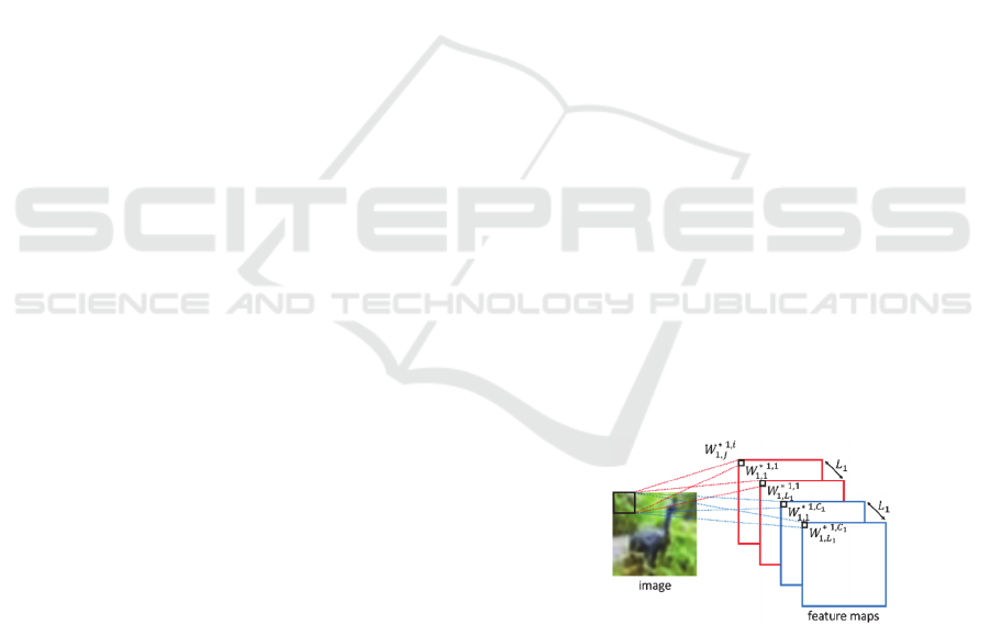
image. The network architecture at the first stage of
our PLSNet is shown in Figure 1. In Figure 1, i and j
of
,
∗,
means the i-th set of local regions and the j-
th filter respectively. The red and blue feature maps
are for a set of the local regions and another set
respectively.
Figure 1: The network architecture at the first stage of our
PLSNet.
2.2 The Second Stage
PLSNet crops a lot of local regions from
feature
maps at the first stage of training images as
explanatory variables, and their class labels are used
as objective variables. Then it does the same
processes as the first stage for each feature map at
the first stage. If the number of components used for
Hierarchical Feature Extraction using Partial Least Squares Regression and Clustering for Image Classification
391
PLS is
, it obtains
feature maps per
image. When we apply clustering to the second stage
too, it obtains
feature maps per image.
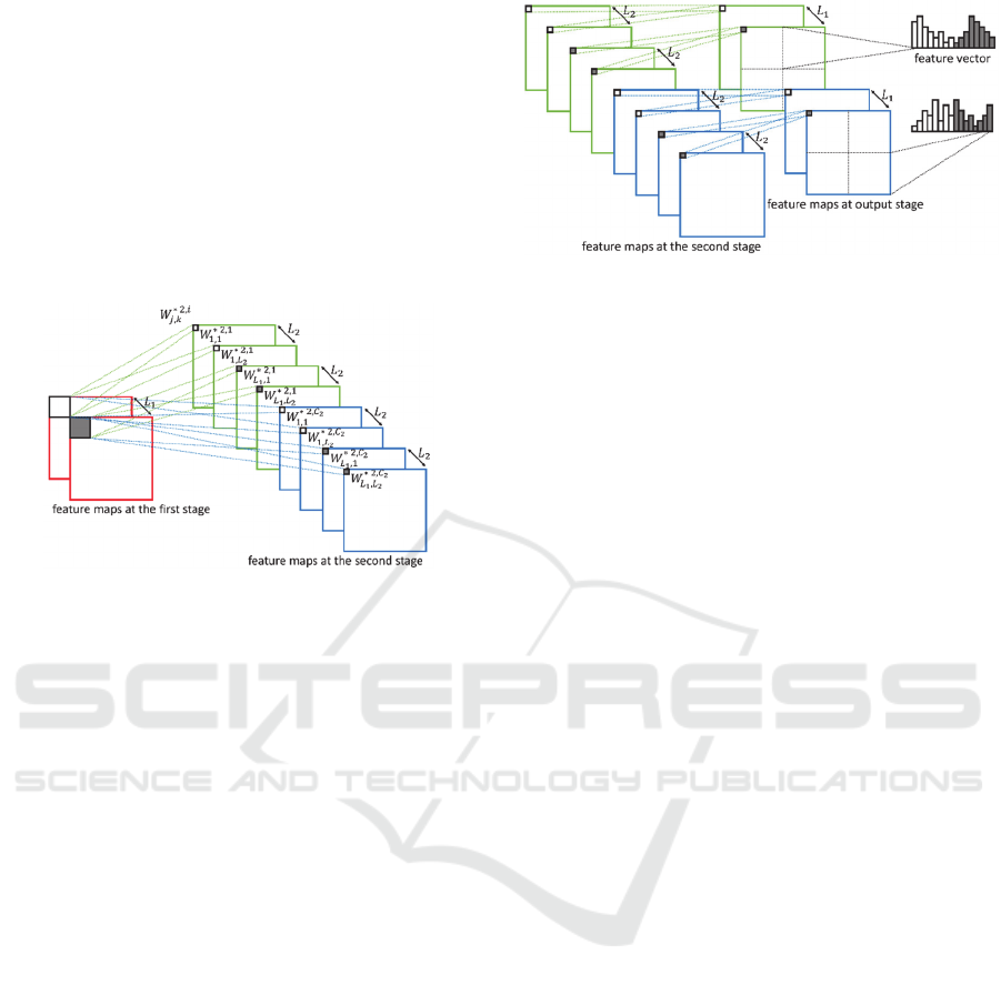
The network architecture at the second stage of our
PLSNet is shown in Figure 2. This figure shows the
network architecture for a set at the first stage. In
Figure 2, i, j and k of
,
∗,
means the i-th set of the
local regions cropped from the feature maps at the
first stage and the k-th filter learned from the j-th
feature maps from training images at the first stage
respectively.
Figure 2: The network architecture at the second stage of
our PLSNet.
2.3 Output Stage
We do the same processes as output stage in
PCANet. There are
feature maps at the second
stage for a feature map at the first stage. It binarizes
the feature maps at the second stage by viewing the
signs of the values. In other words, the value is 1 for
positive and 0 for negative. Then it views the
binary bits as a decimal number and converts the
binary bits into a decimal number as
2
(2)
where
means the i-th feature maps at the second
stage for a feature map at the first stage, and
means the converted feature map. The values are in
the range
0,2
1
. After the processes, it divides
the feature maps into some blocks with overlap and
computes a histogram for each block. The histogram
has 2
bins. Then it concatenates all the histograms
into a feature vector. By doing the processes, it
obtains position invariance within each block. In our
PLSNet, there are
feature vectors per image.
We train
SVM and classify images by voting
the result of SVM. The network architecture at
output stage of our PLSNet is shown in Figure 3.
Figure 3: The network architecture at output stage of our
PLSNet.
3 EXPERIMENTS
This section shows experimental results on the
CIFAR-10 dataset. In section 3.1, we explain the
CIFAR-10 dataset and implementation details. In
section 3.2, we show accuracies when we apply
clustering to only the first stage. In section 3.3, we
show accuracies when we apply clustering to both
the first and second stages. In section 3.4, we
visualize the feature maps obtained by our PLSNet.
3.1 Dataset
The CIFAR-10 is a dataset for general object
recognition. It consists of 10 classes; airplane,
automobile, bird, cat, deer, dog, frog, horse, ship and
truck. Each image is natural RGB with 32 × 32
pixels, and the dataset contains 50,000 training and
10,000 test images. In experiments, we used the last
10,000 training images as validation samples, and
the remaining training images were used as training
samples. We selected the optimal hyper-parameters
such as the number of clusters and the cost of SVM
using the validation samples. After the selections of
hyper-parameters, we evaluated our PLSNet using
original training and test samples.
3.2 Applying Clustering to Only the
First Stage
We evaluated our PLSNet when we applied
clustering to only the first stage. We trained two
PLSNets with different hyper-parameters and
evaluated three kinds of PLSNets; the two PLSNets
and the combination of two PLSNets. The sizes of
the filters at the first and second stage were set to 3
× 3, and the number of components used for the one
of two PLSNets was set to 12 and 8 at the first and
second stages respectively. For another PLSNet, the
VISAPP 2017 - International Conference on Computer Vision Theory and Applications
392
sizes of the filters at the first and second stages were
set to 5 × 5, and the number of components used for
PLS was set to 28 and 8 at the first and second
stages respectively. The size and stride of block at
both output stages were set to 8 × 8 and 4 × 4
respectively. In case of these hyper-parameters, the
dimension of feature vectors are 150,528 and
351,232 respectively for a set of clusters. These
hyper-parameters are the same as PLSNet without
clustering.
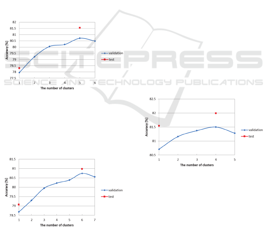
The accuracies of PLSNet whose filter sizes
were set to 3 × 3 are shown in Figure 4. In Figure 4,
1 on the horizontal axis means the PLSNet without
clustering. Figure 4 shows that PLSNet with
clustering obtained 81.54% accuracy when the
number of clusters was set to 5. This accuracy is
3.24% higher than PLSNet without clustering.
According to the accuracies of the validation
samples, the optimal number of clusters was set to 5.
Therefore, we evaluated only PLSNet whose number
of clusters was set to 5 on the test samples.
Figure 4: Accuracy of PLSNet (3 × 3) for varying the
number of clusters at the first stage.
The accuracies of PLSNet whose filter sizes
were set to 5 × 5 are shown in Figure 5. Figure 5
shows that PLSNet with clustering obtained 80.98%
accuracy when the number of clusters was set to 6.
This accuracy is 1.91% higher than PLSNet without
clustering.
Figure 5: Accuracy of PLSNet (5 × 5) for varying the
number of clusters at the first stage.
Furthermore, we evaluated the combined
PLSNet. The dimension of feature vector is 501,760
for a set of clusters. When we combine the feature
vectors, the number of clusters in the two PLSNets
must be the same. From the previous results, we set
the number of clusters to 5. Our PLSNet obtained
82.08% accuracy. This accuracy is 1.35% higher
than the combined PLSNet without clustering. Table
1 shows the best accuracies of each PLSNet with
clustering to only the first stage. The combination of
two PLSNets works well. We found that our PLSNet
improved the accuracies much when we applied
clustering to even only the first stage.
3.3 Applying Clustering to Both the
First and Second Stages
We evaluated our PLSNet when we applied
clustering to both the first and second stages. The
number of clusters at the first stage were decided
from the results in section 3.2.
The accuracies of our PLSNet whose filter sizes
were set to 3 × 3 are shown in Figure 6. In Figure 6,
1 on the horizontal axis means our PLSNet without
clustering at the second stage. From the result in
section 3.2, we set the number of clusters at the first
stage to 5. Figure 6 shows that PLSNet with
clustering obtained 81.99% accuracy when the
number of clusters was set to 4. This accuracy is
3.69% and 0.45% higher than PLSNet without
clustering and PLSNet with clustering to only the
first stage respectively.
Figure 6: Accuracy of PLSNet (3 × 3) for varying the
number of clusters at the second stage.
The accuracies of our PLSNet whose filter sizes
were set to 5 × 5 are shown in Figure 7. From the
result in section 3.2, we set the number of clusters at
the first stage to 6. Figure 7 shows that PLSNet with
clustering obtained 81.65% accuracy when the
number of clusters was set to 4. This accuracy is
2.58% and 0.67% higher than PLSNet without
Hierarchical Feature Extraction using Partial Least Squares Regression and Clustering for Image Classification
393
clustering and PLSNet with clustering to only the
first stage respectively.
Figure 7: Accuracy of PLSNet (5 × 5) for varying the
number of clusters at the second stage.
Furthermore, we evaluated the combined PLSNet.
From the previous results, we set the number of
clusters at the first and second stage to 5 and 3
respectively. Our PLSNet obtained 82.42% accuracy.
This accuracy is 1.69% and 0.34% higher than the
combined PLSNet without clustering and PLSNet
with clustering to only the first stage respectively.
Table 1 shows the best accuracies of each PLSNet
with clustering to both the first and second stages.
We found that our PLSNet improved the accuracies
much when we applied clustering.
We compare our PLSNet with the other methods
in Table 1. Table 1 shows that our PLSNet obtained
the highest accuracies of those methods.
Table 1: Comparison of accuracy (%) of the methods on
the CIFAR-10 dataset.
Methods Accuracy
PCANet (combined) (Chan et al., 2014) 78.67
PLSNet (3×3) (Hasegawa et al., 2016) 78.3
PLSNet (5×5) (Hasegawa et al., 2016) 79.07
PLSNet (combined) (Hasegawa et al.,
2016)
80.73
PLSNet with clustering
to only the 1st stage (3×3)
81.54
PLSNet with clustering
to only the 1st stage (5×5)
80.98
PLSNet with clustering
to only the 1st stage (combined)
82.08
PLSNet with clustering
to both the 1st and 2nd stages (3×3)
81.99
PLSNet with clustering
to both the 1st and 2nd stages (5×5)
81.65
PLSNet with clustering
to both the 1st and 2nd stages (combined)
82.42
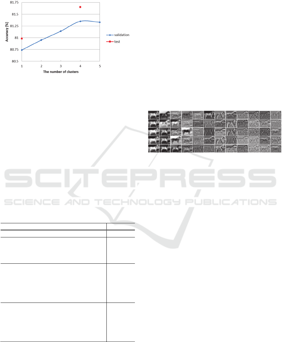
3.4 Visualizing the Feature Maps
Obtained by PLSNet with
Clustering
To validate the effectiveness of our PLSNet, we
visualized the feature maps obtained by PLSNet
with clustering. The feature maps at the first stage
obtained by our PLSNet whose filter sizes were set
to 3 × 3 are shown in Figure 8. The feature maps are
for an image labeled horse. In Figure 8, the
horizontal axis means the number of components
used for PLS, and the vertical axis means the
number of clusters. Figure 8 shows that each
PLSNet obtained a variety of feature maps. We
consider that this is the reason why PLSNet with
clustering obtained higher accuracies than PLSNet
without clustering.
Figure 8: Example of the feature maps obtained by
PLSNet with clustering.
4 CONCLUSIONS
In this paper, we proposed an image classification
method using PLS and clustering. Our PLSNet
obtained higher accuracies than PLSNet without
clustering on the CIFAR-10 dataset.
In the experiments, hyper-parameters used for
PLSNet with clustering were the same as PLSNet
without clustering for fair comparison. In adition, we
used k-means clustering because it is the most basic
methods. Therefore, we will obtain higher
accuracies if we select optimal hyper-parameters and
recent clustering methods. These are subjects for
future works.
REFERENCES
Dudani, S, A., 1976. The distance-weighted k-nearest-
neighbor rule. In IEEE Transactions on Systems, Man,
and Cybernetics.
Vapnik, V., 1998. Statistical learning theory, Wiley. New
York.
Wold, H., 1985. Partial least squares, Wiley. New York.
Hasegawa, R. and Hotta, K., 2016. Plsnet: a simple
network using partial least squares regression for
VISAPP 2017 - International Conference on Computer Vision Theory and Applications
394

image classification. In International Conference on
Pattern Recognition.
Badrinarayanan, V., Kendall, A. and Cipolla, R., 2015.
Segnet: a deep convolutional encoder-decoder
architecture for image segmentation. In International
Conference on Computer Vision.
Krizhevsky, A., Sutskever, I. and Hinton, G. E., 2012.
Imagenet classification with deep convolutional neural
networks. In Advances in Neural Information
Processing Systems 25.
Schwartz, W, R., Kembhavi, A. and Davis, L, S., 2009.
Human detection using partial least squares analysis.
In International Conference on Computer Vision.
Shelhamer, E., Long, J. and Darrell, T., 2015. Fully
convolutional networks for semantic segmentation. In
IEEE Conference on Computer Vision and Pattern
Recognition.
Girshick, R., Donahue, J., Darrell, T. and Malik, J., 2014.
Rich feature hierarchies for accurate object detection
and semantic segmentation. In IEEE Conference on
Computer Vision and Pattern Recognition.
He, K., Zhang, X., Ren, S. and Sun, J., 2014. Spatial
pyramid pooling in deep convolutional networks for
visual recognition. In European Conference on
Computer Vision.
Lecun, Y., Bottou, L., Bengio, Y. and Haffner, P., 1998.
Gradient-based learning applied to document
recognition. In Proceedings of the IEEE.
Oquab, M., Bottou, L., Laptev, I. and Sivic, J., 2014.
Learning and transferring mid-level image
representations using convolutional neural networks.
In IEEE Conference on Computer Vision and Pattern
Recognition.
Taigman, Y., Yang, M., Ranzato, M. and Wolf, L., 2014.
Deepface: closing the gap to human-level performance
in face verification. In IEEE Conference on Computer
Vision and Pattern Recognition.
Chan, T., Jia, K., Gao, S., Lu, J., Zeng, Z. and Ma, Y.,
2014. Pcanet: a simple deep learning baseline for
image classification? In IEEE Transactions on Image
Processing.
Deng, J., Dong, W., Socher, R., Li, L., Li, K. and Fei-Fei,
L., 2009. Imagenet: a large-scale hierarchical image
database. In IEEE Conference on Computer Vision
and Pattern Recognition.
Karpathy, A., Toderici, G., Shetty, S., Leung, T.,
Sukthankar, R. and Fei-Fei, L., 2014. Large-scale
video classification with convolutional neural
networks. In IEEE Conference on Computer Vision
and Pattern Recognition.
Xiao, T., Xu, Y., Yang, K., Zhang, J., Peng, Y. and Zhang,
Z., 2015. The application of two-level attention
models in deep convolutional neural network for fine-
grained image classification. In IEEE Conference on
Computer Vision and Pattern Recognition.
Szegedy, C., Liu, W., Jia, Y., Sermanet, P., Reed, S.,
Anguelov, D., Erhan, D., Vanhoucke, V. and
Rabinovich, A., 2015. Going deeper with
convolutions. In IEEE Conference on Computer
Vision and Pattern Recognition.
Hierarchical Feature Extraction using Partial Least Squares Regression and Clustering for Image Classification
395
