
Modelling and Reasoning with Uncertain Event-observations for
Event Inference
Sarah Calderwood, Kevin McAreavey, Weiru Liu and Jun Hong
School of Electronics, Electrical Engineering and Computer Science, Queen’s University Belfast, Belfast, U.K.
Keywords:
Dempster-Shafer Theory, Event Detection, Event Inference, Uncertain Event-observations.
Abstract:
This paper presents an event modelling and reasoning framework where event-observations obtained from het-
erogeneous sources may be uncertain or incomplete, while sensors may be unreliable or in conflict. To address
these issues we apply Dempster-Shafer (DS) theory to correctly model the event-observations so that they can
be combined in a consistent way. Unfortunately, existing frameworks do not specify which event-observations
should be selected to combine. Our framework provides a rule-based approach to ensure combination occurs
on event-observations from multiple sources corresponding to the same event of an individual subject. In ad-
dition, our framework provides an inference rule set to infer higher level inferred events by reasoning over the
uncertain event-observations as epistemic states using a formal language. Finally, we illustrate the usefulness
of the framework using a sensor-based surveillance scenario.
1 INTRODUCTION AND
RELATED WORK
CCTV surveillance systems are deployed in various
environments including airports (Weber and Stone,
1994), railways (Sun and Velastin, 2003), retail stores
(Brodsky et al., 2001) and forensic applications (Ger-
adts and Bijhold, 2000). Such systems detect, recog-
nise and track objects of interest through gathering
and analysing real-time event-observations from low-
level sensors and video analytic components. This al-
lows the system to take appropriate actions to stop
or prevent undesirable behaviours e.g. petty crime
or harassment. However, event-observations may be
uncertain or incomplete (e.g. due to noisy measure-
ments etc.) while the sensors themselves may be un-
reliable or in conflict (e.g. due to malfunctions, inher-
ent design limitations). As such, an important chal-
lenge is how to accurately model and combine event-
observations from multiple sources to ensure higher
level inferred events that provide semantically mean-
ingful information in an uncertain, dynamic environ-
ment.
In the literature, various event reasoning sys-
tems have been suggested for handling uncertainty in
events (Wasserkrug et al., 2008; Ma et al., 2009). In
particular, the framework proposed by (Wasserkrug
et al., 2008) considers the uncertainty in event-
observations and the uncertainty in rules. Specifi-
cally, this is modelled as a single Bayesian network
which is continuously updated at run-time when new
primitive event-observations are observed. Further-
more, inferred events are continuously recognised us-
ing probabilistic inference over the Bayesian network.
In (Ma et al., 2009; Ma et al., 2010), the authors ad-
dress the problem of uncertain and conflicting infor-
mation from multiple sources. They use Dempster-
Shafer (DS) theory of evidence (Shafer, 1976) to
combine (uncertain) event-observations from multi-
ple sources to find a representative model of the un-
derlying sources. However, in (Ma et al., 2009; Ma
et al., 2010) the authors do not specify what event-
observations to combine. This is necessary to en-
sure combination occurs on event-observations from
multiple sources corresponding to the same event
of an individual subject. If this is not considered
then the combined event-observation result will be
inconsistent and not representative of the underly-
ing sources. Furthermore, in (Ma et al., 2009; Ma
et al., 2010), the authors use a rule-based inference
system to derive inferred events from primitive event-
observations. However, in (Ma et al., 2009; Ma et al.,
2010) they do not define the formal semantics of the
conditions within their inference rules.
The main contributions of this work are as fol-
lows:
(i) We revise and extend significantly the event mod-
elling and reasoning framework of (Ma et al.,
308
Calderwood S., McAreavey K., Liu W. and Hong J.
Modelling and Reasoning with Uncertain Event-observations for Event Inference.
DOI: 10.5220/0006254103080317
In Proceedings of the 9th International Conference on Agents and Artificial Intelligence (ICAART 2017), pages 308-317
ISBN: 978-989-758-220-2
Copyright
c
2017 by SCITEPRESS – Science and Technology Publications, Lda. All rights reserved

2009; Ma et al., 2010) using Dempster-Shafer the-
ory.
(ii) We provide a rule-based approach to specify how
to select the event-observations to be combined.
(iii) We use the framework of (Bauters et al., 2014)
to reason over the uncertain information as prob-
abilistic epistemic states using a formal language.
(iv) We present a scenario from a sensor-based
surveillance system to illustrate our framework.
The remainder of this paper is organised as fol-
lows. In Section 2, we introduce the preliminaries
of DS theory and modelling uncertain information as
epistemic states. In Section 3, we propose our event
modelling and reasoning framework. In Section 4, we
present a sensor-based surveillance scenario to illus-
trate our framework. Finally, in Section 5 we con-
clude this paper and discuss future work.
2 PRELIMINARIES
In this section, we provide the preliminaries on
Dempster-Shafer (DS) theory (Shafer, 1976) and how
to model uncertain information as epistemic states.
2.1 Dempster-Shafer Theory
Dempster-Shafer theory is capable of dealing with in-
complete and uncertain information.
Definition 1. Let Ω be a set of exhaustive and mutu-
ally exclusive hypotheses, called a frame of discern-
ment. A function m : 2
Ω
→ [0, 1] is called a mass func-
tion over Ω if m(
/
0) = 0 and
∑
A⊆Ω
m(A) = 1. Also,
a belief function and plausibility function from m, de-
noted Bel and Pl, are defined for each A ⊆ Ω as:
Bel(A) =
∑
B⊆A
m(B),
Pl(A) =
∑
A∩B6=
/
0
m(B).
Any A ⊆ Ω such that m(A) > 0 is called a fo-
cal element of m. Intuitively, m(A) is the propor-
tion of evidence that supports A, but none of its strict
subsets. Similarly, Bel(A) is the degree of evidence
that the true hypothesis belongs to A and Pl(A) is the
maximum degree of evidence supporting A. The val-
ues Bel(A) and Pl(A) represent the lower and upper
bounds of belief, respectively.
To reflect the reliability of evidence we can apply
a discounting factor to a mass function using Shafer’s
discounting technique (Shafer, 1976) as follows:
Definition 2. Let m be a mass function over Ω and
α ∈ [0,1] be a discount factor. Then a discounted
mass function with respect to α, denoted m
α
, is
defined for each A ⊆ Ω as:
m
α
(A) =
(1 − α) · m(A), if A ⊂ Ω,
α + (1 − α) · m(A), if A = Ω.
The effect of discounting is to remove mass as-
signed to focal elements and to then assign this mass
to the frame. When α = 0, the source is completely
reliable, and when α = 1, the source is completely un-
reliable. Once a mass function has been discounted,
it is then treated as fully reliable.
One of the best known rules to combine mass
functions is Dempster’s rule of combination, which
is defined as follows:
Definition 3. Let m
i
and m
j
be mass functions over
Ω from independent and reliable sources. Then the
combined mass function using Dempster’s rule of
combination, denoted m
i
⊕ m
j
, is defined for each
A ⊆ Ω as:
(m
i
⊕ m
j
)(A) =
c
∑
B∩C=A
m
i
(B)m
j
(C), if A 6=
/
0,
0, otherwise,
where c =
1
1−K(m
i
,m
j
)
is a normalization constant with
K(m
i
,m
j
) =
∑
B∩C=
/
0
m
i
(B)m
j
(C).
The effect of the normalization constant c, with
K(m
i
,m
j
) the degree of conflict between m
i
and m
j
,
is to redistribute the mass value assigned to the empty
set.
To reflect the belief distributions from precondi-
tions to the conclusion in an inference rule, in (Liu
et al., 1992), a modelling and propagation approach
was proposed based on the notion of evidential map-
ping Γ.
Definition 4. Let Γ : Ω
e
× 2
Ω
h
→ [0,1] be an eviden-
tial mapping from frame Ω
e
to frame Ω
h
that satisfies
the condition Γ(ω
e
,
/
0) = 0 and
∑
H⊆Ω
h
Γ(ω
e
,H) = 1.
Let Ω
e
and Ω
h
be frames, with m
e
a mass function
over Ω
e
and Γ an evidential mapping from Ω
e
to Ω
h
.
Then a mass function m
h
over Ω
h
is an evidence prop-
agated mass function from m
e
with respect to Γ and
is defined for each H ⊆ Ω
h
as:
m
h
(H) =
∑
E⊆Ω
e
m
e
(E)Γ
∗
(E,H),
where: Γ
∗
(E,H) =
i, if H 6=
S
H
E
∧ ∀ω
e
∈ E, Γ(ω
e
,H) > 0,
1 − j, if H =
S
H
E
∧ ∃ω
e
∈ E, Γ(ω
e
,H) = 0,
1 − i + j if H =
S
H
E
∧ ∀ω
e
∈ E,Γ(ω
e
,H) > 0,
0, otherwise,
Modelling and Reasoning with Uncertain Event-observations for Event Inference
309

with i =
∑
ω
e
∈E
Γ(ω
e
,H)
|E|
, j =
∑
H
0
∈H
E
Γ
∗
(E,H
0
), H
E
=
{H
0
⊆ Ω
h
| ω
e
∈ E, Γ(ω
e
,H
0
) > 0} and
S
H
E
= {ω
h
∈
H
0
| H
0
∈ H
E
}.
2.2 Modelling Uncertain Information as
Epistemic States
To define an epistemic state we let At be a finite
set of propositional atoms. Then for a set of atoms
A ⊆ At, the set of literals given the atoms in A are:
lit(A) = {a|a ∈ A} ∪ {¬a|a ∈ A}. A formula φ is de-
fined in Backus-Naur Form (BNF) as φ ::= a|¬a|(φ
1
∧
φ
2
)|(φ
1
∨φ
2
) where all formulas are in Negation Nor-
mal Form (NNF). Here, the language is denoted as
L . A function ω : At → {T RUE,FALSE} is called
a possible world (or interpretation) which assigns a
truth value to every variable. The set of all possible
worlds is denoted Ω. A possible world ω is a model
of a formula φ iff the possible world ω makes φ true in
the standard truth functional way, denoted as ω |= φ.
The set of all models of φ is denoted as mod(φ). An
epistemic state is defined as follows:
Definition 5. (from (Ma and Liu, 2011)) Let Ω be a
set of possible worlds. An epistemic state is a map-
ping Φ : Ω → Z ∪ {−∞,+∞}.
An epistemic state represents the state of the world
where Φ(ω) represents the degree of belief in a possi-
ble world ω. Then Φ(ω) = +∞ indicates ω is fully
plausible, Φ(ω) = −∞ indicates ω is not plausible
and Φ(ω) = 0 indicates total ignorance about ω. For
ω,ω
0
∈ Ω and Φ(ω)>Φ(ω
0
) then ω is more plausible
than ω
0
.
To reason about epistemic states we consider the
work of (Bauters et al., 2014). The language L is ex-
tended with the connectives > and ≥ such that we
have φ>ψ and φ ≥ ψ respectively. The former means
φ is strictly more plausible than ψ whereas the latter
means φ is at least as plausible as ψ. The resulting lan-
guage L
∗
can be defined in BNF as φ ::= a|¬a|φ
1
∧
φ
2
|φ
1
∨ φ
2
|φ
1
>φ
2
|φ
1
≥ φ
2
where φ
1
is strictly more
plausible than φ
2
if φ
1
>φ
2
. Moreover, φ
1
is more
plausible or equal to φ
2
if φ
1
≥ φ
2
.
The semantics of the language L
∗
are defined us-
ing a mapping λ where formulas φ ∈ L
∗
map onto
Z ∪ {−∞,+∞}. Intuitively, λ(φ), associated with the
formula φ reflects how plausible it is. However, if φ is
not a propositional statement (i.e. φ /∈ L ) it becomes
necessary to pare down the formula until it becomes
a classical propositional statement. This is completed
by the following definition:
Definition 6. (from (Bauters et al., 2014)) Let φ ∈ L
∗
be a formula in the extended language. Then when
φ ∈ L, λ(φ) = max{Φ(ω)|ω |= φ} with max(
/
0) = −∞.
Otherwise, we define λ(φ) = λ(pare(φ)) with pare de-
fined as:
pare(φ ∧ ψ) = check(φ) ∧ check(ψ)
pare(φ ∨ ψ) = check(φ) ∨ check(ψ)
pare(φ ≥ ψ) =
> if λ(φ) ≥ λ(ψ)
⊥ otherwise
pare(φ>ψ) =
> if λ(φ)>λ(ψ)
⊥ otherwise
pare(notφ) =
> if φ ∈ L and λ(¬φ) ≥ λ(φ)
⊥ otherwise
check(φ) =
φ if φ ∈ L
pare(φ) otherwise
with > a tautology (i.e. true) and ⊥ an inconsistency
(i.e. false).
The intuition of paring down is straightforward:
for the operators ∧ and ∨ we verify if it is a formula
in the language L . Otherwise, we need to pare it down
to get a propositional formula. When the operator is
either > or ≥, we define it as φ>ψ which is read as
’φ is more plausible than ψ’ or ’we have less reason
to believe ¬φ than ¬ψ’. This will always evaluate to
true or false, i.e. > or ⊥.
Using the λ-mapping we now define when a for-
mula φ is entailed.
Definition 7. (from (Bauters et al., 2014)) Let Φ be
an epistemic state and φ a formula in L
∗
. We say that
φ is entailed by Φ, written as Φ |= φ, if and only if
λ(φ)>λ(¬φ).
3 REASONING ABOUT
UNCERTAIN
EVENT-OBSERVATIONS
In this section we propose a new event modelling and
reasoning framework by revising and extending the
framework of (Ma et al., 2009; Ma et al., 2010). Ini-
tially, we formally define an event model to represent
the attributes and semantics of event-observations de-
tected from information provided by various sources.
This ensures that the event-observations themselves
are represented and reasoned as well as allowing in-
ferences to be made subsequently. Events can be clas-
sified as (i) external events which are those directly
gathered from external sources or (ii) inferred events
which are the result of the inference rules of the event
model.
ICAART 2017 - 9th International Conference on Agents and Artificial Intelligence
310

3.1 Event Detection
Let ϒ be a non-empty finite set of variables. The
frame (or set of possible values) associated with a
variable υ ∈ ϒ is denoted Ω
υ
. For a set of vari-
ables Ψ ⊆ ϒ, the (product) frame Ω
Ψ
is defined as
∏
υ∈Ψ
Ω
υ
.
Definition 8. Let [t,t
0
] be an interval of time start-
ing at timepoint t and ending at timepoint t
0
, s be
a source, p be a subject, Ψ be a set of variables
and m be a mass function over Ω
Ψ
. Then a tuple
e = ([t,t
0
],s, p,m) is called an event-observation.
The mass function m represents some (uncertain)
event-observation, made by source s at its temporal
location [t,t
0
], for some real-world event. We assume
that a source can only make one event-observation at
timepoint t about an individual subject p
1
. Further-
more, a source can detect multiple event-observations
at any one time as long as they correspond to different
subjects.
Definition 9. Let S be a set of sources. A function r :
S 7→ [0,1] is called a source reliability measure such
that r(s) = 1 if s is completely reliable, r(s) = 0 if s is
completely unreliable and r(s) ≥ r(s
0
) if s is at least
as reliable as (s
0
).
Information related to event-observations are
modelled as mass functions. However, due to their
reliability we apply their source reliability measure
to derive discounted mass functions that can then be
treated as fully reliable. The reliability measure of
each source is based on its historical data, age, de-
sign limitations and faults etc. A primitive event set
E
P
will contain a set of event-observations e
1
...e
n
with their corresponding discounted mass functions
m
α
1
...m
α
n
.
Example 1. Consider two independent sources s
1
and
s
2
where s
1
is CCTV which detects the behaviour of a
subject named Alice (Ω
Ψ
b
= {walking,sitting}) and
is 90% reliable and s
2
is a thermometer which de-
tects the temperature of a room (Ω
Ψ
t
= {0,...,50})
and is 85% reliable. Information has been obtained
from 9 am such that s
1
:[walking(80% certain)] and
s
2
[30
o
C]. By modelling the (uncertain) informa-
tion as mass functions we have m
1
({walking}) =
0.8, m
1
(Ω
Ψ
b
) = 0.2 and m
2
({30}) = 1, respectively.
Given this information we have the following event-
observations in E
P
:
1
We use ” − ” to denote an event-observation that does
not have a subject.
e
1
= ([900,901],s
1
,Alice,m
0.1
1
({walking}) = 0.72,
m
0.1
1
(Ω
Ψ
b
) = 0.28),
e
2
= ([900,902],s
2
,−,m
0.15
2
({30}) = 0.85,
m
0.15
2
(Ω
Ψt
) = 0.15).
For these event-observations we apply the discount
factors (i.e. α = 0.1 and 0.15 respectively) for s
1
and
s
2
to the mass functions m
1
and m
2
to obtain the dis-
counted mass functions.
Definition 10. An event model M is defined as a tuple
hE
P
,E
C
,E
I
i where E
P
is a primitive event set (a set
of discounted event-observations), E
C
is a combined
event set (a set of combined event-observations) and
E
I
is an inference event set (a set of inferred events).
3.2 Event-observation Combination
Constraints
In some situations, we need to combine mass func-
tions which relate to different attributes. However,
combination rules require that mass functions have
the same frame. The vacuous extension is a tool used
for defining mass functions on a compatible frame.
A mass function m
Ω
Ψ
1
, expressing a state of belief
on Ω
Ψ
1
is manipulated to a finer frame Ω
Ψ
n
, a refine-
ment of Ω
Ψ
1
using the vacuous extension operation
(Wilson, 2000), denoted by ↑. The vacuous extension
of m
Ω
Ψ
1
from Ω
Ψ
1
to the product frame Ω
Ψ
1
× Ω
Ψ
n
,
is obtained by transferring each mass m
Ω
Ψ
1
, for any
subset A of Ω
Ψ
1
to the cylindrical extension of A.
Definition 11. Let Ψ
1
,Ψ
n
be sets of variables and
m
1
,...,m
n
be mass functions over frames Ω
Ψ
1
,Ω
Ψ
n
.
Then by vacuous extension, we obtain mass functions
over Ω
Ψ
1
×···×Ψ
n
, denoted m
Ω
Ψ
1
↑(Ω
Ψ
1
×···×Ω
Ψ
n
)
where
m
Ω
Ψ
1
↑(Ω
Ψ
1
×···×Ω
Ψ
n
)
(B) =
m
Ω
Ψ
1
(A), if B = A × Ω
Ψ
2
× ··· × Ω
Ψ
n
,
A ⊆ Ω
Ψ
1
0, otherwise.
Here, the propagation brings no new evidence and
the mass functions are strictly equivalent (in terms of
information).
Event-observations detected from various sources
relating to a specific feature or subject identification
will be combined at time T . The original and most
common method of combining mass functions is us-
ing Dempster’s combination rule. However, other
combination operators such as the context-dependent
combination rule from (Calderwood et al., 2016) or
the disjunctive combination rule from (Dubois and
Prade, 1992) may be more suitable given the infor-
mation obtained from the sources.
Modelling and Reasoning with Uncertain Event-observations for Event Inference
311

Definition 12. Let {e
1
,...,e
n
} be a set of observa-
tions from E
P
and {t,...,t
0
} be a set of timepoints
in T from e
1
,...,e
n
. Then the combined observation
e
1
◦ ··· ◦ e
n
is defined as:
([min(T
min
),max(T
max
)],s
1
∧ · ·· ∧ s
n
,m
0
1
⊕ · ·· ⊕ m
0
n
),
where [min(T
min
),max(T
max
)] represents the mini-
mum and maximum of the set of timepoints, m
0
i
=
m
↑Ψ
1
×···×Ψ
n
i
and m
0
i
= m
1−r(s
1
)
i
. Given that each m
0
i
is
a discounted mass function, we have that r(s
1
∧ ··· ∧
s
n
) = 1.
Notably, we can combine event-observations
when their time interval overlaps. When this occurs,
we select the earliest (resp. latest) timepoint from the
events to use as timepoint t (resp. t
0
) of the com-
bined event-observation. For example, assume event-
observations e
1
and e
2
are detected at [900,905] and
[902,907] respectively. Then, the interval of time for
a combined event-observation is [900,907].
However, before a combination occurs we need to
decide which event-observations are selected to com-
bine.
Definition 13. An event-observation constraint rule c
is defined as a tuple
c = (T S,S, p)
where T S is a time span constraint, S is a set of
sources whose mass functions are to be combined
from event-observations in E
P
and p is a subject that
is assigned to event-observations.
In this work, we consider time, source and subject
constraints. We combine event-observations obtained
from multiple sources when they relate to the same
event of an individual subject and are within a rea-
sonable time span
2
. For example, event-observations
relating to a subject p from sources s
1
and s
2
will be
combined if they have been obtained at the same time.
Example 2. Consider the following constraint rules
in the event-observation constraint rule set:
c
1
= (5,{s
1
,s
3
}, p);
c
2
= (0,{s
2
,s
4
,s
5
,s
6
},−).
Assume we have six independent sources s
1
,...,s
6
where
(i) event-observations from sources s
1
and s
3
are ob-
tained (at 9:00:35 am and 9:00:40 am respec-
tively) about a subject named Alice;
(ii) event-observations from s
2
, s
4
, s
5
and s
6
are ob-
tained (at 9 am) about the thermometers observing
themselves.
2
This will be domain-specific.
Given the event-observations from (i), the constraint
rule c
1
is selected to combine the event-observations
from sources s
1
and s
3
as the timespan is within 5
seconds and they relate to a subject named Alice. Fur-
thermore, given the event-observations from (ii), the
constraint rule c
2
is selected to combine the event-
observations from sources s
2
, s
4
, s
5
and s
6
as they
were all obtained at 9 am and they relate to the same
type of source i.e. thermometers.
The semantics for combining event-observations
is as follows:
Definition 14. Let c be an event-observation con-
straint rule, hE
P
,E
C
,E
I
i be the event model and E ⊆
E
P
be a set of event-observations. Then the event-
observation combination with respect to c be defined
as:
E ∧ c 6|=⊥ s.t.∀E
0
⊂ E,E
0
∧ c |=⊥
hE
P
,E
C
,E
I
i → hE
P
\E, E
C
∪ {e
1
◦ · ·· ◦ e
n
},E
I
i
combine.
3.3 Event Inference
Event inferences are expressed as a set of inference
rules which are used to represent the relationship
between primitive and combined event-observations.
New inferred events are derived which are more
meaningful and highly significant. For example, a
person entering a building at night may imply its ei-
ther a staff member or an unauthorised person. How-
ever if further event-observations are obtained and
combined where the person is a male with their face
obscured then it may imply a higher level threat such
as a theft.
In our framework, an epistemic state is instanti-
ated to a mass function as follows:
Definition 15. (adapted from Definition 5) Let Ω be
a set of possible worlds. An epistemic state is a map-
ping Φ : 2
Ω
→ Z ∪ {−∞, +∞}.
In this paper, we define an inference rule as fol-
lows:
Definition 16. An inference rule i is defined as a tuple
i = (T S,φ, Γ
Φ
Ψ
)
where TS is the time span, φ ∈ L
∗
is a formula and
Γ is a multi-valued mapping that propagates a mass
function from an epistemic state in Ω
Φ
to a new mass
function in Ω
Ψ
.
Notably, Ω
ϒ
and Ω
Ψ
are some product frames for
sets of variables ϒ and Ψ, respectively (as in the first
paragraph of Section 3.1). Moreover, L
∗
is the lan-
guage defined over the same set of attributes (atoms)
where a condition is always a formula in L
∗
. Here,
a formula can be equivalent to a possible world when
ICAART 2017 - 9th International Conference on Agents and Artificial Intelligence
312

there is a conjunction of literals. Thus, an inference
rule defines a condition over some set of attributes and
then uses evidential mapping to propagate the mass
function from the possible worlds Φ of an epistemic
state to the new mass function (that is related to a dif-
ferent set of attributes). The latter will be included in
the new inferred event.
We will now explore the inference rule in more
detail.
A: Formula - φ
Initially, we have a set of possible worlds Ω and
a mass function over Ω (which is domain-specific).
Relevant mass functions (from discounting or vacu-
ous extension (see Definition 11) are then combined
using Dempster’s rule to provide a combined mass
function.
Example 3. Let A
1
and A
2
be independent attributes
where Ω
1
= {a, b} and Ω
2
= {p,q} are their possible
values, respectively. Let m
1
and m
2
be mass functions
over Ω such that:
m
1
({a}) = 0.72,m
1
(Ω
1
) = 0.28,
m
2
({p}) = 0.765,m
2
(Ω
2
) = 0.235.
By vacuously extending Ω
1
with Ω
2
we obtain Ω
1
×
Ω
2
= {(a, p),(a, q),(b, p),(b,q)}. Then by vacuously
extending m
1
and m
2
to mass functions over Ω
1
×Ω
2
,
we have:
m
1
({(a, p),(a,q)}) = 0.72,m
1
(Ω
1
× Ω
2
) = 0.28,
m
2
({(a, p),(b, p)}) = 0.765,m
2
(Ω
1
× Ω
2
) = 0.235.
By combining the new mass functions m
1
and m
2
us-
ing Dempster’s rule we have a new combined mass
function m as follows:
m({(b, p),(a, p)}) = 0.214,m({(a, p)}) = 0.551,
m({(a,q),(a, p)}) = 0.169, m(Ω
1
× Ω
2
) = 0.066.
To evaluate the formulas we use the plausibility
function from DS theory. The justification being that
possibilistic logic uses the possibility measure, and
the possibility measure in possibility theory is com-
parable to the plausibility function in DS theory. As
such, we instantiate Definition 6 and Definition 7 as
follows: λ(φ) = Pl(φ) = Pl(mod(φ)) where the λ-
mapping has been instantiated with the plausibility
function. This means, by definition, we have that
Pl(>) = 1 and Pl(⊥) = 0.
Example 4. (Continuing Example 3) Let A
1
= a,
A
2
= p and A
1
= a ∧ A
2
= p be formulas
3
. Then
(i) mod(A
1
= a) = {(a, p),(a,q)},
(ii) mod(A
2
= p) = {(a, p),(b, p)},
3
Assume ordering (A
1
,A
2
).
(iii) mod(A
1
= a ∧ A
2
= p) = {(a, p)},
(iv) mod(¬(A
1
= a ∧A
2
= p)) = {(a, q),(b, p)(b,q)}.
The plausibility values for the formulas are:
(i) Pl(A
1
= a) =1,
(ii) Pl(A
2
= p) =1,
(iii) Pl(A
1
= a ∧ A
2
= p) = 1,
(iv) Pl(¬(A
1
= a ∧ A
2
= p)) = 1.
Then Pl(A
1
= a ∧ A
2
= p) 6> Pl(¬(A
1
= a ∧ A
2
= p)).
The formula A
1
= a ∧ A
2
= p is not entailed.
B: Evidential mapping - Γ
Φ
Ψ
Evidential mappings are defined from a mass
function in an epistemic state Ω
Φ
to a new mass func-
tion in Ω
Ψ
. These mappings allow us to derive a mass
function to be included as part of the new inferred
event.
Example 5. Consider Table 1 where Ω
Ψ
=
{c
1
,c
2
,c
3
} represents conclusion 1, conclusion 2 and
conclusion 3, respectively.
Table 1: Evidential mapping Γ
Φ
Ψ
from Ω
Φ
=
{(a, p), (a,q),(b, p),(b,q)} to Ω
Ψ
= {c
1
,c
2
,c
3
}.
{c
1
} {c
1
,c
2
} {c
2
,c
3
} {c
3
}
(a, p) 0.5 0.5 0 0
(a,q) 0 0 1 0
(b, p) 0 0 0.7 0.3
(b,q) 0 0 0.5 0.5
From the evidential mapping in Table 1 and the
combined mass function (from Example 3), then a
mass function m
Ψ
over Ψ is the evidence propagated
mass function from m
Φ
with respect to Γ such that:
m
Ψ
({c3}) = 0.045,m
Ψ
({c1,c2}) = 0.38,
m
Ψ
({c1}) = 0.38,m
Ψ
({c2,c3}) = 0.196.
Example 6. Let i
1
be an inference rule. Then we
have:
i
1
= (0,(A
1
= a ∧ A
2
= p),Γ
Φ
Ψ
).
where Γ
Φ
Ψ
is an evidential mapping as shown in Ta-
ble 1.
The semantics of event inference is defined as fol-
lows:
Definition 17. Let i be an inference rule, φ be the for-
mula from i, hE
P
,E
C
,E
I
i be the event model, E ⊆ E
P
∪
E
C
∪ E
I
be a set of event-observations from the primi-
tive event set, combined event set and inference event
set respectively. Then the inference rule selection with
respect to i be defined as:
E |= φ
hE
P
,E
C
,E
I
i → hE
P
,E
C
,E
I
∪ {e
I
1
,...,e
I
n
i
in f er.
Modelling and Reasoning with Uncertain Event-observations for Event Inference
313
Notably, an inferred event e
I
i
will be defined sim-
ilar to that of a primitive event-observation (see Def-
inition 8) except that in this case its mass function is
an evidence propagated mass function and its source
will be a set of sources.
Now, we can extend the definition of the event
model M as follows:
Definition 18. An event model M
∗
is defined as a tu-
ple hE
P
,E
C
,E
I
,C,Ii where C is an event-observation
combination constraints rule set, I is an inference rule
set and the other items are the same as those defined
in Definition 10.
Figure 1: An illustration of the event model M
∗
using prim-
itive and combined event-observations to infer an inferred
event.
4 SURVEILLANCE SYSTEM
SCENARIO
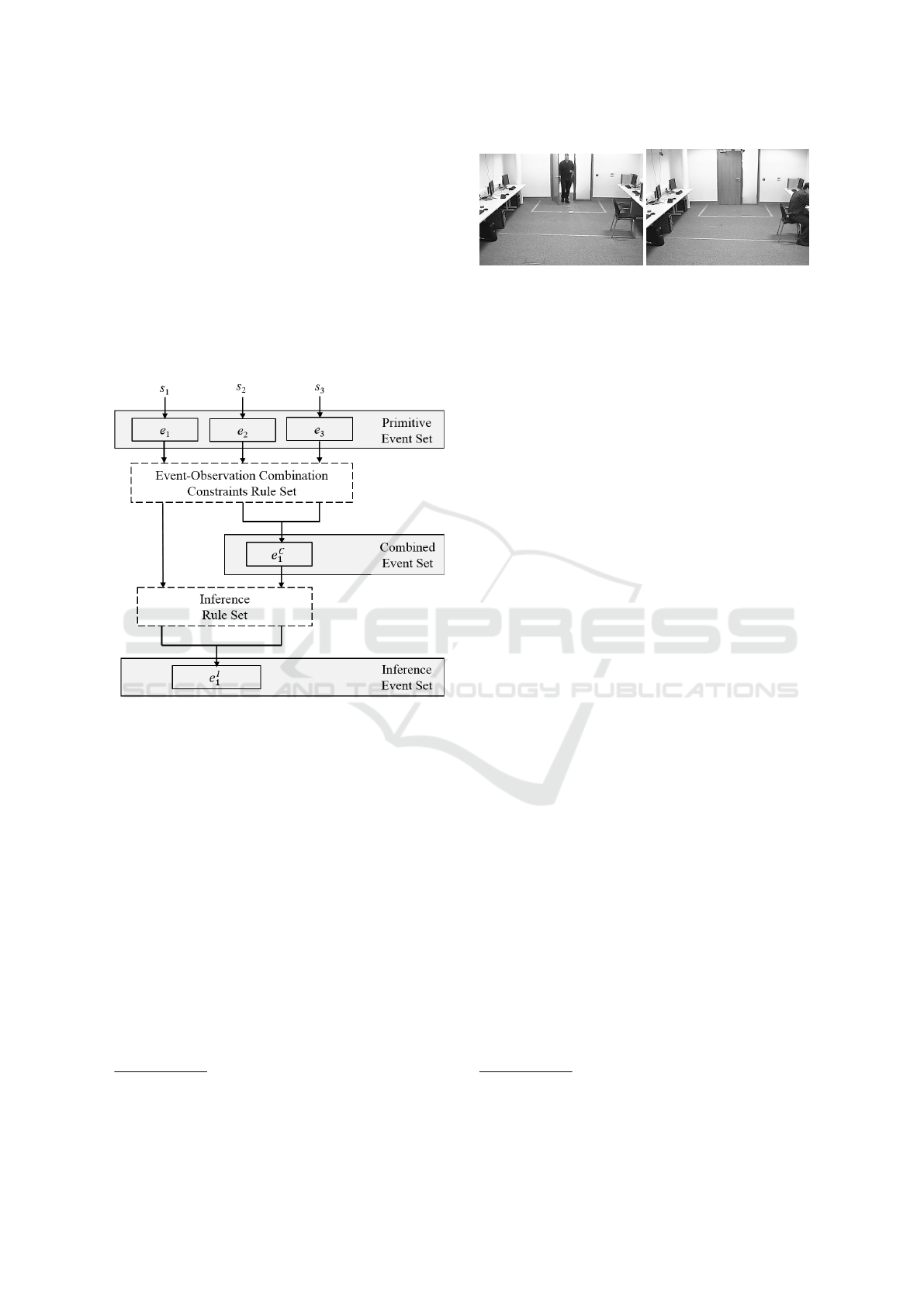
In this section, we consider a scenario from a surveil-
lance system to illustrate our event modelling and rea-
soning framework. Specifically, we monitor a single
subject
4
i.e. a staff member enter a computer room at
10 am by swiping their access card (see Figure 2 (i)).
Information is retrieved for that staff member and they
are assigned an id e.g. p
1
,..., p
n
. Within the room,
the staff member will fulfil their job therefore their
behaviour is expected to coincide with their job role.
For example, a technician may enter the room, walk
towards a computer, sit down at a computer and ac-
cess the network. However, a cleaner may enter the
4
For multiple subjects, algorithms for video classifica-
tion or tracking etc. will detect each individual subject and
assign an unique id.
Figure 2: A staff member (i) entering a computer room and
(ii) sitting at a computer.
room, walk towards a computer and dust the desk. A
violation will occur if the behaviour of that staff mem-
ber does not match that expected of their job. For
example, given Figure 2 (ii) it shows a staff member
sitting at the computer. This behaviour is normal for
a technician but a violation for a cleaner.
4.1 Event Detection
4.1.1 Primitive Event-observations
In the surveillance system, a number of heteroge-
neous sources with various levels of granularity (e.g.
cameras, microphones) will identify and monitor
the behaviour of each staff member through clas-
sification analysis etc. Sources s
1
, s
2
and s
3
are
cameras located within the computer room where
source s
1
detects the obfuscation of a staff member
i.e. Ω
o
= {obscured,¬obscured} and is 90% reli-
able, s
2
detects the gender of a staff member i.e.
Ω
g
= {male, f emale} and is 70% reliable and s
3
de-
tects the behaviour of a staff member i.e. Ω
b
=
{walking, sitting}
5
and is 90% reliable. Furthermore,
sources s
4
and s
5
are light sensors which detect light
in the computer room i.e. Ω
l
= {on,o f f }. These
sources are 60% and 90% reliable, respectively. In
this scenario, we assume the event-observations from
sources s
1
, s
2
and s
3
were obtained from 10 am for
a subject p
1
and from sources s
4
and s
5
for the light
sensor. We have:
s
1
: [obscured(80%certain)],
s
2
: [male(70%certain)],
s
3
: [walking(80%certain)],
s
4
: [on(70%certain)],
s
5
: [on(90%certain)].
By modelling the (uncertain) information as mass
5
Notably, the behaviour of a staff mem-
ber can be extended to the following: Ω
b
=
{walking,sitting,running,standing,loitering,...}
ICAART 2017 - 9th International Conference on Agents and Artificial Intelligence
314

functions we have:
m
1
({obscured}) = 0.8, m
1
(Ω
Ψ
o
) = 0.2,
m
2
({male}) = 0.7,m
2
(Ω
Ψ
g
) = 0.3,
m
3
({walking}) = 0.8, m
3
(Ω
Ψ
b
) = 0.2,
m
4
({on}) = 0.7,m
4
(Ω
Ψ
l
) = 0.3,
m
5
({on}) = 0.9,m
5
(Ω
Ψ
l
) = 0.1.
Given this information we have the following primi-
tive event-observations in E
P
:
e
1
= ([1000,1001],s
1
, p
1
,m
0.1
1
({obscured}) = 0.72,
m
0.1
1
(Ω
Ψ
o
) = 0.28)),
e
2
= ([1000,1001],s
2
, p
1
,m
0.3
2
({male}) = 0.49,
m
0.3
2
(Ω
Ψg
) = 0.51)),
e
3
= ([1001,1002],s
3
, p
1
,m
0.1
3
({walking}) = 0.72,
m
0.1
3
(Ω
Ψb
) = 0.28)),
e
4
= ([1000,1015],s
4
,−,m
0.4
4
({on}) = 0.42,
m
0.4
4
(Ω
Ψl
) = 0.58)),
e
5
= ([1000,1015],s
5
,−,m
0.1
5
({on}) = 0.81,
m
0.1
5
(Ω
Ψl
) = 0.19)).
Notably, we have applied the discount factors (i.e. α
= 0.1, 0.3, 0.1, 0.4 and 0.1 respectively) for sources
s
1
,...s
5
to obtain the discounted mass functions for
the event-observations e
1
,...,e
5
respectively.
In a real world surveillance system, event-
observations will be continuously detected about each
subject over a period of time. As such, further event-
observations may include the following for the subject
p
1
:
e
6
= ([1002,1015],s
3
, p
1
,m
0.1
3
({sitting}) = 0.72,
m
0.1
3
(Ω
Ψb
) = 0.28)),
e
7
= ([1002,1002],s
7
, p
1
,m
0.1
6
({wakeup}) = 0.72,
m
0.1
6
(Ω
Ψn
) = 0.28)),
e
8
= ([1003,1015],s
7
, p
1
,m
0.1
7
({login}) = 0.72,
m
0.1
7
(Ω
Ψn
) = 0.28)),
···
Here, the event-observation e
6
shows that source
s
3
detects the subject p
1
sitting. Furthermore, the
event-observations e
7
and e
8
relate to the network
events i.e. Ω
n
= {wakeup, sleep,login,logo f f } de-
tected by s
7
which is 90% reliable. In both of these
event-observations the information obtained was 80%
certain. It is also worth noting that further event-
observations can be obtained to account for the real
complexity in a working surveillance system e.g. con-
sidering other sensor information on multiple subjects
(obtained from multiple sources) and from various
measurement devices.
4.1.2 Event-observation Combination
Constraints Rule Set
Consider the following rules:
c
1
= (60,{s
1
,s
2
}, p
1
),
c
2
= (0,{s
4
,s
5
},−).
The rule c
1
states that event-observations from
sources s
1
and s
2
will be combined if there time span
is within 60 seconds and they correspond to the same
event for a staff member p
1
. The rule c
2
states that
event-observations from sources s
4
and s
5
will be
combined if they have been obtained at the same
time. Notably, in this scenario s
3
is not combined
with other sources therefore we do not need a rule.
6
4.1.3 Combined Event-observations
In the surveillance system, it becomes necessary to
define mass functions onto the same frame. By vacu-
ously extending Ω
Ψ
o
with Ω
Ψ
g
we obtain
Ω
Ψ
o
,Ψ
g
= Ω
Ψ
o
× Ω
Ψ
g
=
{(obscured,male),(obscured, f emale),
(¬obscured,male),(¬obscured, f emale)}.
By using the constraint rule c
1
and Dempster’s com-
bination rule we obtain m
1
⊕ m
2
for subject p
1
, re-
sulting in the following combined observation m
C
1
in
E
C
:
e
C
1
= ([1000,1001],{s
1
,s
2
}, p
1
,
m
C
1
({(¬obscured,male), (obscured,male)}) = 0.137,
m
C
1
({(obscured,male)}) = 0.353,
m
C
1
({(obscured, f emale),(obscured,male)}) = 0.367,
m
C
1
(Ω
o
× Ω
p
) = 0.143.
Notably, sources s
4
and s
5
will not be combined with
sources s
1
and s
2
as s
4
and s
5
are from different
sources, they do not correspond to the same event and
they are not associated with subject p
1
.
By using the constraint rule c
2
and Dempster’s
combination rule we obtain m
4
⊕ m
5
for the ther-
mometer readings, resulting in the following com-
bined observation m
C
2
in E
C
:
e
C
2
= ([1000,1015],{s
4
,s
5
},−,
m
C
2
({on}) = 0.89,m
C
2
(Ω
l
) = 0.11).
6
In the real world, s
3
will be combined with multiple
sources to detect the behaviour of a subject.
Modelling and Reasoning with Uncertain Event-observations for Event Inference
315

4.2 Event Inference
4.2.1 Inference Rules
In the surveillance system we have inference rules
such as the following:
i
1
= (0,(ob f uscation = obscured∧
gender = male ∧ behaviour = walking), Γ
Φ
Ψ
),
i
2
= (0,(ob f uscation = obscured∧
gender = male ∧ behaviour = sitting), Γ
Φ
Ψ
),
i
3
= (0,(light = on), Γ
Φ
1
Ψ
2
),
where Γ from Ω
Φ
={(obscured,male,walking),...,
(¬obscured, f emale,sitting)} to Ω
Ψ
= {l,m,h}
which represents the threat classifications of low
level, moderate level and high level, respectively.
The rule i
1
states that if an obscured male is cur-
rently walking then it infers a moderate-high level
threat (or an obscured male walking). The next rule
i
2
states that if an obscured male is sitting at the com-
puter then it infers a high level threat (or an obscured
male sitting at a computer). Notably, further rules can
be added to this rule set to infer further events of inter-
est. For example, given the event-observations e
6
, e
7
and e
8
we could have a rule to state that an obscured
male is sitting at a computer and has logged on to the
network.
Let ob f uscation, gender, behaviour be attributes,
(denoted as O, G and B, respectively) where Ω
o
=
{obscured,¬obscured}, Ω
g
= {male, f emale} and
Ω
b
= {walking,sitting} are their possible values (de-
noted as Ω
o
= {o,¬o}, Ω
g
= {m, f } and Ω
b
= {w,s},
respectively). Let O = o, G = m, B = w and O =
o ∧ G = m ∧ B = w be formulas
7
. Then:
(i) mod(O = o) =
{(o,m,w),(o,m,s),(o, f ,w),(o, f , s)},
(ii) mod(G = m) =
{(o,m,w),(o,m,s),(¬o,m,w),(¬o,m,s)},
(iii) mod(B = w) =
{(o,m,w),(o, f ,w),(¬o,m,w),(¬o, f , w)},
(iv) mod(O = o ∧ G = m ∧ B = w) =
{(o,m,w)},
(v) mod(¬(O = o ∧ G = m ∧ B = w)) =
{(o,m,s),...,(¬o, f ,w)}.
The plausibility values for the formulas are:
(i) Pl(O = o) = 1,
(ii) Pl(G = m) = 1,
7
Assume ordering (O,G,B).
(iii) Pl(B = w) = 1,
(iv) Pl(O = o ∧ G = m ∧ B = w) = 1,
(v) Pl(¬(O = o ∧ G = m ∧ B = w)) = 1.
Then Pl(O = o∧G = m∧B = w) 6> Pl(¬(O = o∧G =
m ∧ B = w)). The formula O = o ∧ G = m ∧ B = w is
not entailed.
Alternatively, consider the light attribute (denoted
as L) where Ω
l
= {on,o f f }. Let L = on be a formula.
Then the set of models are:
(i) mod(L = on) = {(on)},
(ii) mod(¬(L = on)) = {(o f f )}.
The plausibility values for the formulas are:
(i) Pl(L = on) = 1,
(ii) Pl(¬(L = on)) = 0.11.
Then Pl(L = on) > Pl(¬(L = on)) as 1 > 0.11. The
formula L = on is entailed.
Table 2: Evidential mapping from Ω
Φ
=
{(o,m,w), ... ,(¬o, f , s)} to Ω
Ψ
= {l,m,h}.
{l} {l, m} {m} {m,h} {h}
(o,m,w) 0 0 0.25 0.75 0
(o,m,s) 0 0 0 0.6 0.4
(o, f , w) 0 0 0.25 0.75 0
(o, f , s) 0 0 0 0.6 0.4
(¬o,m,w) 1 0 0 0 0
(¬o,m,s) 0.9 0.1 0 0 0
(¬o, f , w) 1 0 0 0 0
(¬o, f , s) 0.9 0.1 0 0 0
Given the evidential mapping from Table 2 and
the combined mass function, then a mass function m
Ψ
over Ψ is the evidence propagated mass function from
m
Φ
with respect to Γ such that:
m
Ψ
({m,h}) = 0.648,m
Ψ
({h}) = 0.054,
m
Ψ
({l,m}) = 0.003,m
Ψ
({l}) = 0.167,
m
Ψ
({m}) = 0.189.
Given the event-observations obtained from
10 am, we have the following inferred event in E
I
:
e
I
1
= ([1000,1015],{s
1
,s
2
,s
3
}, p
1
,
m
I
1
({m,h}) = 0.648,m
I
1
({h}) = 0.054,
m
I
1
({l,m}) = 0.003,m
I
1
({l}) = 0.167,
m
I
1
({m}) = 0.189).
5 CONCLUSION
In this paper we have presented an event mod-
elling and reasoning framework to represent and rea-
son with uncertain event-observations from multiple
ICAART 2017 - 9th International Conference on Agents and Artificial Intelligence
316

sources such as low-level sensors. This approach
provides rule-based systems to specify which event-
observations to combine as well as to infer higher
level inferred events from both primitive and com-
bined event-observations. We demonstrate the appli-
cability of our work using a real-world surveillance
system scenario. In conclusion, we have found that
it is important to correctly model, select and com-
bine uncertain sensor information so that we obtain
inferred events that are highly significant. This en-
sures appropriate actions can be taken to stop or pre-
vent undesirable behaviours that may occur. As for
future work, we plan to deal with partially matched
information in the formula (condition) of inference
rules. In other words, if a formula of a rule is met,
this rule is triggered and an inferred event is gener-
ated. However, if a formula of multiple rules are par-
tially met, then we need an approach to decide which
rule should be triggered.
REFERENCES
Bauters, K., Liu, W., Hong, J., Sierra, C., and Godo, L.
(2014). Can(plan)+: Extending the operational se-
mantics for the BDI architecture to deal with uncertain
information. In Proceedings of the 30th International
Conference on Uncertainty in Artificial Intelligence,
pages 52–61.
Brodsky, T., Cohen, R., Cohen-Solal, E., Gutta, S., Lyons,
D., Philomin, V., and Trajkovic, M. (2001). Visual
surveillance in retail stores and in the home. Advanced
video-based surveillance systems, pages 50–61.
Calderwood, S., McAreavey, K., Liu, W., and Hong,
J. (2016). Context-dependent combination of sen-
sor information in Dempster-Shafer Theory for BDI.
Knowledge and Information Systems.
Dubois, D. and Prade, H. (1992). On the combination
of evidence in various mathematical frameworks. In
Flamm, J. and Luisi, T., editors, Reliability Data Col-
lection and Analysis, pages 213–241. Springer.
Geradts, Z. and Bijhold, J. (2000). Forensic video investi-
gation. In Multimedia Video-Based Surveillance Sys-
tems, pages 3–12. Springer.
Liu, W., Hughes, J., and McTear, M. (1992). Represent-
ing heuristic knowledge in DS theory. In Proceedings
of the 8th International Conference on Uncertainty in
Artificial Intelligence, pages 182–190.
Ma, J. and Liu, W. (2011). A framework for manag-
ing uncertain inputs: An axiomization of reward-
ing. International Journal of Approximate Reasoning,
52(7):917–934.
Ma, J., Liu, W., and Miller, P. (2010). Event modelling and
reasoning with uncertain information for distributed
sensor networks. In Scalable Uncertainty Manage-
ment, pages 236–249. Springer.
Ma, J., Liu, W., Miller, P., and Yan, W. (2009). Event com-
position with imperfect information for bus surveil-
lance. In Advanced Video and Signal Based Surveil-
lance, 2009. AVSS’09. Sixth IEEE International Con-
ference on, pages 382–387. IEEE.
Shafer, G. (1976). A Mathematical Theory of Evidence.
Princeton University Press.
Sun, B. and Velastin, S. (2003). Fusing visual and audio in-
formation in a distributed intelligent surveillance sys-
tem for public transport systems .
Wasserkrug, S., Gal, A., and Etzion, O. (2008). Inference
of security hazards from event composition based on
incomplete or uncertain information. In IEEE Trans-
actions on Knowledge and Data Engineering, pages
1111–1114.
Weber, M. and Stone, M. (1994). Low altitude wind shear
detection using airport surveillance radars. In Radar
Conference, 1994., Record of the 1994 IEEE National,
pages 52–57. IEEE.
Wilson, N. (2000). Algorithms for Dempster-Shafer the-
ory. In Handbook of Defeasible Reasoning and Uncer-
tainty Management Systems. Springer Netherlands.
Modelling and Reasoning with Uncertain Event-observations for Event Inference
317
