Chat Based Contact Center Modeling

System Modeling, Parameter Estimation and Missing Data Sampling

Per Enqvist

and G

oran Svensson

1,2

Division of Optimization and Systems Theory, Kungliga Tekniska H

ogskolan, Lindstedtsv 25, Stockholm, Sweden

Teleopti WFM, Teleopti AB, Stockholm, Sweden

Keywords:

Queueing, Chat, Chat-based Queueing Systems, Parameter Estimation, Gibbs Sampling.

Abstract:

A Markovian system model for a contact center chat function is considered and partially validated. A hypoth-

esis test on real chat data shows that it is reasonable to model the arrival process as a Poisson process. The

arrival rate can be estimated using Maximum likelihood. The service process is more involved and the estima-

tion of the service rate depends on the number of simultaneous chats handled by an agent. The estimation is

made more difﬁcult by the low level of detail in the given data-sets. A missing data approach with Gibbs sam-

pling is used to obtain estimates for the service rates. Finally, we try to capture the generalized behaviour of

the service-process and propose to use generalized functions to describe it when little information is available

about the system at hand.

1 INTRODUCTION

Contact centers usually offer several types of media

to enable customer communication. Chat function-

ality is one such type of media that in recent years

has grown in popularity. This stresses the importance

of good modeling and parameter estimations for chat

based systems.

In this paper a Markovian chat system model is

considered (Enqvist and Svensson, 2017). The chat

system is viewed as a queue-based state-space model,

akin to traditional queueing systems of inbound tele-

phone call centers, described in detail elsewhere such

as in (Koole, 2013; Gans et al., 2003; Aksin et al.,

2007). However, chat systems behave slightly differ-

ent than traditional telephone queues in that an agent

can work with several customers simultaneously. We

make the assumption that the number of customers

an agent is serving effects the service rate with which

the service is provided. A queueing based state-space

model should capture both how many customers each

agent is currently serving and how many customers

there are in the system in total, as well as the varying

service rates.

The main goals of this paper are to argue that such

a queueing-based state-space model is reasonable, to

support such a model by use of real world data and

to propose methods for estimating the rate parameters

for a chat system from real but incomplete data-sets.

The quality and level of detail of the underlying

data can severely limit the choice of methods and the

uncertainty of estimates. When there exist limitations

on available data it may be necessary to rely more on

prior information and thus we propose that general

parameterized functions are used to lower the vari-

ance of the estimates by including empirical informa-

tion about chat systems general behaviour.

Due to the strong dependence on data we propose

a data classiﬁcation structure that pertains to chat sys-

tems. The classiﬁcation of underlying data would in-

dicate which technique is appropriate. The accuracy

and choice of any, realistic, model will be data de-

pendent. For a statistical analysis of a call center see

(Brown et al., 2005).

It is natural to divide the problem into two parts,

one part for the arrival rate process and one for the

service rate process. The former lends itself to stan-

dard methods of estimation when the level of detail of

the underlying data is good enough. While the latter

often leads to complications due to data on aggregated

or mean value form, i.e., low level of detail.

We show that it is reasonable to describe the ar-

rival process in terms of a homogeneous Poisson pro-

cess on 15-minute or 30-minute intervals. We sup-

port this position by χ

-square hypothesis testing at

ﬁve percent signiﬁcance level on two data-sets. For

more on nonhomogeneous arrival processes we refer

to (Green and Kolesar, 1991) and (Whitt, 2007).

464

Enqvist P. and Svensson G.

Chat Based Contact Center Modeling - System Modeling, Parameter Estimation and Missing Data Sampling.

DOI: 10.5220/0006251604640469

In Proceedings of the 6th International Conference on Operations Research and Enterprise Systems (ICORES 2017), pages 464-469

ISBN: 978-989-758-218-9

When estimating at the service rate process the sit-

uation gets more complicated. One possible cause

of complications occur if the start and ﬁnish times

of chat dialogues are not recorded. In our data-sets

only the number of initiated chats per agent and in-

terval is available. Since an agent can serve several

customers in parallel we make the assumption that

the service per customer is a non-increasing func-

tion in the number of currently served customers. In

(Bekker et al., 2004) the authors explore varying ser-

vice levels and in (Bekker et al., 2011) adapting ser-

vice rates are investigated. In computer systems pro-

cessor sharing is a common phenomena, see (Cohen,

1979). Our model is inspired by both the previous

situations, where an agent has capacity to perform si-

multaneous tasks but at varying rates. A further com-

plication is due to data often only being available on

an aggregated level. Thus it is not possible to dis-

cern the actual (pointwise) workload distribution for

the interval. We suggest a missing data approach,

via the expectation maximation algorithm and Gibbs

sampling, to handle this problem.

There might also exist general information about

the system, such as how likely it is that there are cus-

tomers waiting in the queue and the arrival rate from

a previous estimation. One might also include data

from other chat systems and assume that there are

similarities. Hence we propose to model service rate

per customer as a continuous non-increasing func-

tion, depending on the state of the chat system and

the speciﬁc agent. Such a function can provide an-

swers about the maximum allowed chats in parallel to

fullﬁll some quality of service goal, like maximizing

throughput through the system or to support stafﬁng

decisions.

In Section 2, data is discussed and the data-sets are

presented. In Section 3, the proposed queueing-based

state-space model is introduced and parametrized.

The parameters to be estimated are also stated. In

Section 4, the estimation models for the arrival pro-

cess is explained and the hypothesis testing is show

for speciﬁc data-sets. Also the missing data approach

for estimation of the service rates is presented.

2 DATA CHARACERISTICS

What can be achieved in terms of reliable estimates, in

a contact center environment, is highly dependent on

the amount and quality of the available data. There-

fore, it makes sense to categorize data in terms of

quality. We identify three major aspects that deter-

mine the overall quality and three subsets that are im-

portant for estimations in queueing systems, namely:

1. Number of data records, 2. The level of detail,

3. Relevant data-sets. The data-sets can be split into

general system, agent speciﬁc and customer speciﬁc

data.

The number of data records is an important factor

in determining the level of accuracy of estimates. The

level of detail determines how easily one can perform

estimations. Furthermore, in the context of queue-

ing systems, it is meaningful to differentiate between

three types of data-subsets. The ﬁrst set concerns

data on a system level, such as offered load per inter-

val. The second subset pertains to agent speciﬁc data,

data like agent-id and number of initiated chat dia-

logues per interval. The third subset of data records

contain information on individual customers, such as

customer-id, arrival time to the system and waiting

time in queue.

In cases where there are few data records, low de-

tail level or when not all three subcategories are avail-

able leads to uncertainty in the estimations. This type

of uncertainty has to be managed, which motivates

why we need methods to provide reliable estimates in

the face of poor data quality.

The given data-sets, on which this paper is based,

come in two subsets, where the ﬁrst subset contain

general queue data and the second contain agent spe-

ciﬁc data. Thus customer speciﬁc data is missing

in all cases. The data deemed useful in the context

of this paper is presented, while other data posts not

deemed to inﬂuence the procedings is supressed.

After discussing the matter with responsible data

base administrators it is found that the data is not

completely machine generated and thus may contain

errors due to human factors. This type of problem

requires serious attention but for the purposes of this

text it is ignored apart from some pre-processing with

respect to outliers and records with low information

content.

2.1 General Queue Related Data

In the ﬁrst type of data subset the important data posts

are the ones representing date, intraday intervals and

offered load. The data is given per date and per in-

terval, thus we introduce d ∈ D = {1, ... ,D} index-

ing the days, i ∈ I = {1, ... ,I} indexing the intraday

intervals and w

∈ {1, . . . ,W } index the day of the

week, where W = 7. Let N

d,i

∈ N represent the num-

ber of arrivals on day d in interval i, i.e., offered load.

The notation was inspired by (Gans et al., 2009).

Chat Based Contact Center Modeling - System Modeling, Parameter Estimation and Missing Data Sampling

465

2.2 Agent Speciﬁc Data

In the second type of data subset the important data

posts are the ones representing date, intraday interval,

agent identity, number of initialized chats and aggre-

gated time spent with open chat dialogues. The time

spent chatting is the sum of all chat dialogues, thus

the total time can be greater than the length of the

corresponding interval.

2.3 Customer Speciﬁc Data

Many contact centers neglect to record customer spe-

ciﬁc data, such as arrival time, time waiting, time in

service, service provided by agent-id, time of aban-

donment, etc. When such level of detail exists it is

straight forward to estimate service rates and related

parameters. The customer speciﬁc data-sets are miss-

ing for the chat systems investigated in this paper.

2.4 Given Data-Sets

Information of given data-sets. The size is measured

as the raw data text ﬁle size.

Table 1: Given data-sets.

Data-set Syst. data Ag. data Size

TA: queue yes no 5.3 MB

TA: agent no yes 49.7 MB

TC: queue1 yes no 3.5 MB

TC: queue2 yes no 2.3 MB

TC: agent no yes 8.4 MB

Where TA is a large travel agent company and TC

is a large telecom company. Syst. data is short for

System data and Ag. data is short for Agent data.

3 STATE-SPACE QUEUEING

MODEL DESCRIPTION

The queue-based system considered here is approx-

imated by a Markovian state-space model that is de-

scribed in detail in (Enqvist and Svensson, 2017). The

states represent the total number of customers in the

system, the number of agents working during that in-

terval and also contains information about the num-

ber of customers that each agent is currently serving,

possibly up to some maximum number. We refer to

(Asmussen, 2003) for queueing theory in general.

State transition rates are determined by new ar-

rivals and completed service sessions. New arrivals

are either placed in a common queue or start recieving

service from an available agent according to a routing

rule.

Completed services depend on the number of

agents, the number of customers in parallel that each

agent is serving and the corresponding service rates

according to a generalized processor sharing model,

as in (Cohen, 1979), for each agent.

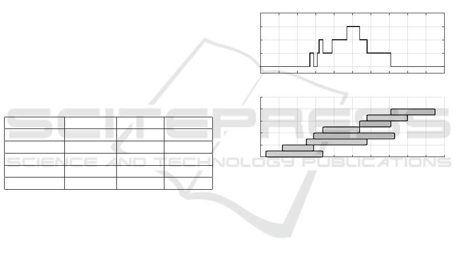
An example, of a chat queue with one agent and a

maximum of three jobs in parallel, is shown in Figure

1. The lower chart shows the jobs as they are seen

by the agent. When a new job starts recieving service

the number of customers waiting in line, if any, drops

by one, as seen in the top ﬁgure. The example can be

expanded to include more agents which, together with

exponential service times and Poisson arrivals, quite

naturally gives rise to a Markovian state-space model.

time

0 1 2 3 4 5 6 7 8 9 10

Waiting queue

One Agent System, max 3 parallel chats

time

0 1 2 3 4 5 6 7 8 9 10

Jobs

Jobs being handled

Figure 1: An example of a one agent chat queue. In the

upper graph the number of customers currently waiting in

queue is depicted. In the lower chart the different jobs are

shown, from the time they start recieving service until they

leave the system. The maximum number of customers that

can be served in parallel, in this example, is three.

3.1 The Arrival Process

New customers enter the system according to an ar-

rival process that is assumed to be Poisson with pa-

rameter λ

, where w

correspond to the day of the

week and i to the interval. We assume that arrivals

are independent and identically distributed. That this

is a reasonable assumption is demonstrated in Section

4.1, as part of the model validation process.

Newly arrived customers either have to wait in line

or are assigned an agent according to the routing rule.

In this paper they are routed to the agent with the least

number of customers in service. In the case that there

are more than one agent serving the same, least num-

ber, of customers then random selection is used.

ICORES 2017 - 6th International Conference on Operations Research and Enterprise Systems

466

3.2 The Service Process

The service rates of the agents can be studied per

agent, by groups of agents or by assuming all agents

perform at the same rate of service. The two former

situations require more data and can cause the under-

lying state-space to grow extremly large, hence in this

paper we choose to treat all agents as equivalent. It

might also be considered that agents provide the same

kind of service during different intraday intervals or it

may be assumed that the service rates vary depend-

ing on the interval. The latter case requires more data

and may be impractical due to the need to solve many

versions of the system.

The state of an agent will be taken as the number

of currently served customers in parallel, possibly up

to some maximum number.

Furthermore, we assume that the service times of

the agents are exponentially distributed with rate pa-

rameters µ

, where j ∈ {0, 1, . . . ,m} represents the

number of currently served customers. These service

rates are dependent on the state of the agent and rep-

resent the fact that an agent serving several customers

simultaneously cannot devote the same type of atten-

tion to all of them as to a single customer.

The service times of the agents are assumed to be

independent of each other and identically distributed,

only depending on the number of customers in par-

allel. Here we assume that the different customers

served by the same agent at the same time are inde-

pendent.

In Section 4.2, we consider the estimation of the

service rates of the agents.

4 PARAMETER ESTIMATION

AND MODEL VALIDATION

This section will be divided into two major parts, the

ﬁrst account for the arrival process and the validity of

the Poisson assumption and the second part consid-

ers the service process and the estimation of the ser-

vice rates for the agents, subject to varying numbers

of chats in parallel.

4.1 The Arrival Process

Data is given on the form of date, 15- or 30-minute

interval and offered load, i.e., number of arrivals N

d,i

per day and interval. We collect all data-points per-

taining to each day of the week and intraday interval

in a vector, denoted by ˜a

of length L

All the { ˜a

}:s are then pre-processed by remov-

ing outliers and entire vectors that contain too little in-

formation. Let { ¯a

} denote the resulting processed

set of vectors, now containing only trusted data. As-

suming that the arrivals are independent and identi-

cally distributed and specifying the likelihood func-

tion to be the joint function for all observations in the

speciﬁed vector ¯a

L(λ

; ¯a

) = f (a

,. . . , a

|λ

). (1)

varies from vector to vector depending on the

given data-set. Then a maximum likelihood esti-

mation (MLE) of the Poisson parameter can be per-

formed to obtain the corresponding arrival rate per in-

terval and day of the week. The estimation is unbiased

and given by the sample mean (Haight, 1967, Ch. 5)

∑

l=1

. (2)

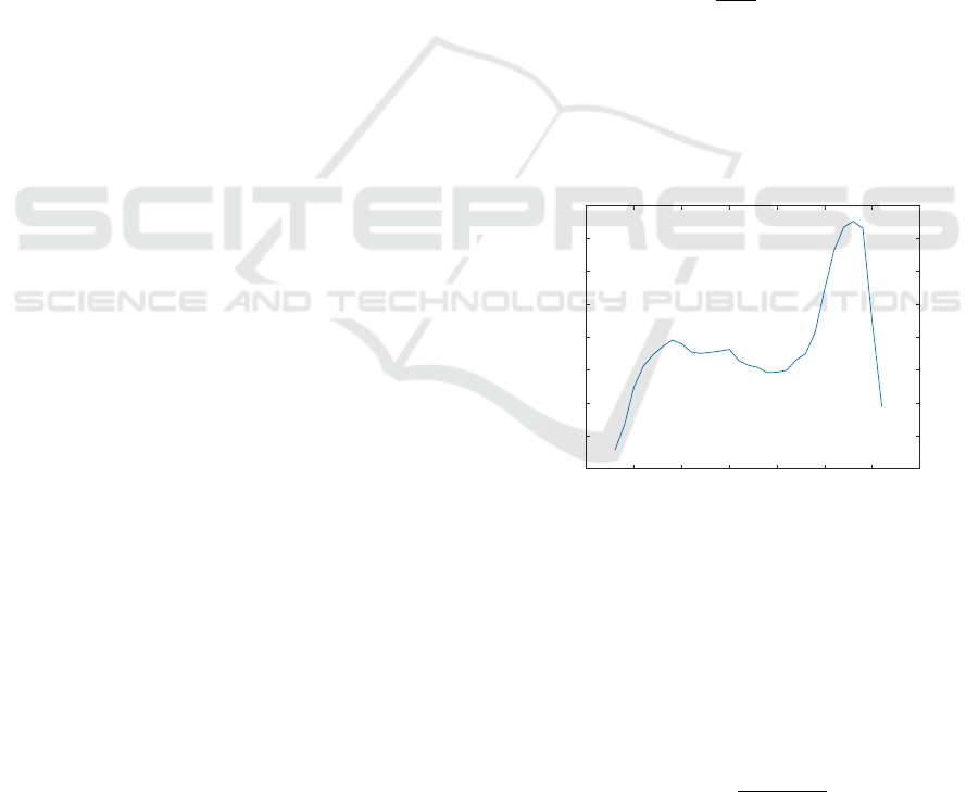
An example of estimated arrival rates for a chat

system of a travel agency are shown in Figure 2.

The actual arrival rates have been modiﬁed by request

from the company, but the general behaviour is cap-

tured. It is shown for 30-minute intervals.

Intervals, [30min]

10 15 20 25 30 35 40 45

Arrival rate,

100

One week day arrival rate estimation

Figure 2: MLE of the arrival rates for one day of the week

with half hour intervals. (Rates are modiﬁed by request

from the company).

A common assumption for many queueing sys-

tems is that arrivals can be modeled by a homoge-

neous Poisson process. To show that this is plausible

the data is tested via a Pearson χ

-test, with test statis-

tic given by

∑

i=1

− E

)

(3)

where n represents the maximum observation value

category, O

the number of observations of type i and

the expected number of observations of type i. The

Chat Based Contact Center Modeling - System Modeling, Parameter Estimation and Missing Data Sampling

467

null hypothesis, H

, is deﬁned to be that data is Pois-

son distributed with parameter

, and the test is

performed at 5% signiﬁcance level.

Examining the data-sets it is found that the as-

sumed Poisson arrival rate is not rejected for the ma-

jority of the intervals and day of the week, results

given in Table 2.

Table 2: Example showing the number of non-rejected and

rejected H

-hypothesises for two different pre-processings

of the same 15-minute interval data-sets.

Data Pre-process Not rejected Rejected

TA Low 277 110

TA High 260 52

TC2 Low 232 210

TC2 High 232 46

The intervals for which the Poisson assumption is

rejected are mostly found in the beginning and at the

end of the day. When the data is aggregated into half

hour intervals the frequency of rejections decrease.

In Table 2 it can be seen that the result is dependent

on the pre-processing of the data, thus non-automated

data processing was needed to obtain the results. In-

formation to this end was supplied by the data-base

administrators.

Considering the results we ﬁnd it reasonable to

model the arrivals as a Poisson process for the intents

and purposes of this work, for a similar but detailed

paper see (Brown et al., 2005)

4.2 The Service Process

The queue and service are modelled as a Markov pro-

cess, where the service rates of each agent depends on

the number of current clients. To decide if this model

assumption is reasonable we would like to perform a

hypothesis test. However, such a test could be per-

formed in the full information case, where client data

is available, but for the given data sets such a test is

not easily performed.

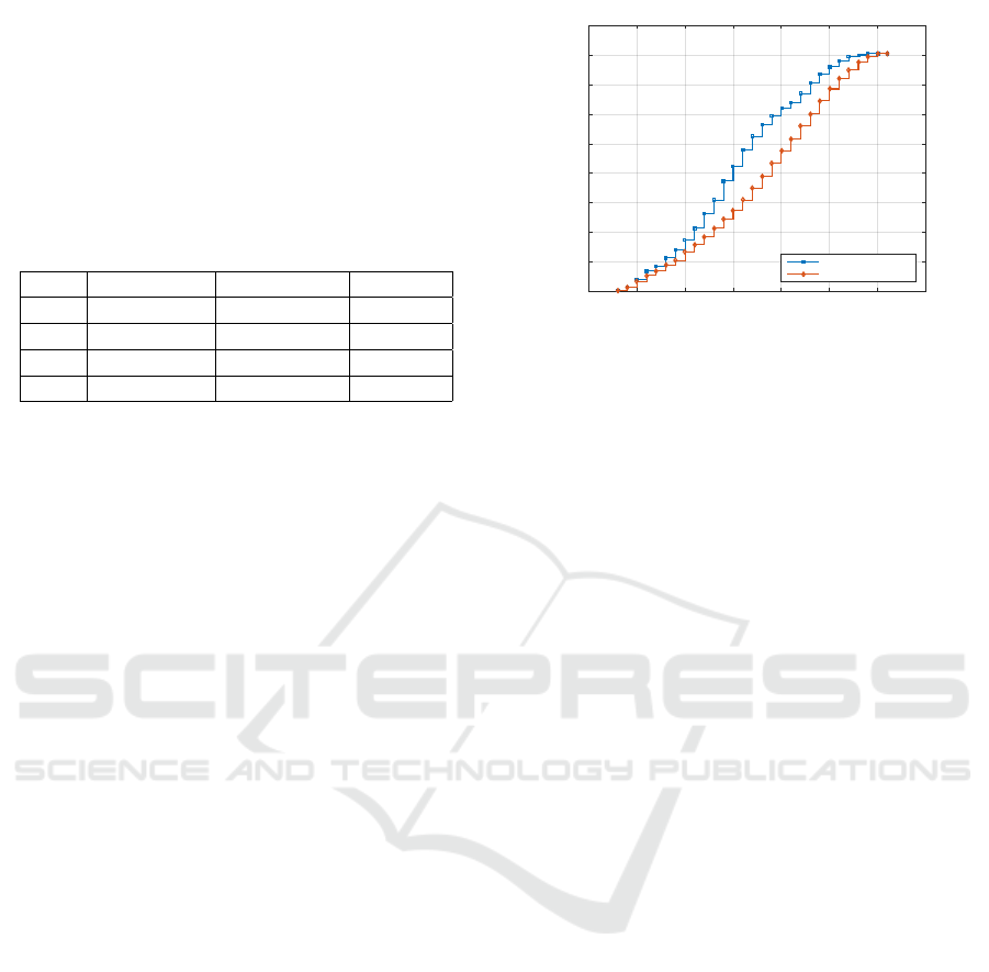
To illustrate the difﬁculties arising from data on

an aggregated format we introduce an example case

as can be seen in Figure 3, were the cumulative ar-

rivals and the cumulative number of answered chats

is shown. Note that only the interval in which arrivals

and answered chats occur is known.

Assuming that the model setup is suitable, we con-

centrate on the problem to estimate the various service

intensities of the agents.

For the full data case the intensities can be esti-

mated from information about the state transitions of

the system, by using a MLE method. However, the

given data-sets lack this level of detail and a direct

MLE is not feasible.

Interval

10 15 20 25 30 35 40 45

Cumulative counts

100

120

140

160

180

Cumulative chat arrivals and answered chats

Cumulative Arrivals

Cumulative Answered

Figure 3: Example showing the cumulative number of ar-

rivals and answered chats for a chat queue where data is

aggregated per interval.

One approach is to try to estimate the missing data

ﬁrst and then apply the MLE approach. Consider one

agent over a sequence of time windows i = 1,·· · , n in

I. Let x

denote the information about block i needed

to determine the MLE, and let y

denote the informa-

tion about block i that is observable, i.e., the informa-

tion provided by the considered data set. Assume that

θ contains all the unknown intensities µ

. It would

be very difﬁcult, or even impossible, to determine a

closed form expression for the probability of observ-

ing the provided data given the intensities θ, i.e., for

1:n

). Here, y

1:n

denotes the values of y

to y

Therefore, we propose to apply the expectation max-

imization (EM) algorithm (Moon, 1996) and (Demp-

ster et al., 1977) to determine the estimate of θ. Start-

ing from an initial guess θ

we want to determine

Q(θ;θ

) = E

[logPr

1:n

)|y

1:n

], (4)

for the expectation step of the EM algorithm. To

take the expectation under θ

it is necessary to have

1:n

). It can be determined using single site

Gibbs sampling (Gelfand and Smith, 1990) where

we should make use of the given observable data.

Sequentially determine Pr

1:i−1

i+1:n

1:n

) for

each i = 1, · ·· , n. If y

1:n

contains information about

the number of arrivals and working time in the blocks

it should be used to determine the probabilities. Thus

we need the x

:s to contain the missing informa-

tion needed to determine the intensities. Let x

,. . . , B

,. . . , T

}, where d

represents the

number of ﬁnished chats in interval i, B

are the inter-

departure times, T

the inter-arrival times and `

the

number of new arrivals in interval i, which is observ-

able. The maximum number of customers in block i is

bounded by the number of customers at the beginning

of the interval, N

, and the number of arrivals during

the interval `

. Let z

= {x

1:i−1

i+1:n

1:n

}, then the

ICORES 2017 - 6th International Conference on Operations Research and Enterprise Systems

468

conditional probabilities

Pr(x

) =

∑

j=1

Pr(x

= j)Pr(d

= j|z

), (5)

can be determined. These correspond to all possible

combinations of jumps in an interval.

The ﬁnal piece is to use that we can observe the to-

tal chat time in interval i. This impose a linear equal-

ity constraint on the variables in x

In the maximization step of the EM algorithm an

updated estimate θ

is determined from

= argmax

Q(θ;θ

). (6)

This process is repeated until sufﬁcient conver-

gence has been achieved.

4.3 Proposed Service Rate Function

In order to reduce the number of parameters to esti-

mate we propose that a parametric function represen-

tation of the service rate is used. This function class

can be chosen to represent physical properties of the

rate parameters. We propose the following function

class.

f ( ˜n) =

(

0, ˜n < 1

˜na



1 −

1+be

c(d−˜n)



, ˜n ≥ 1

(7)

where ˜n ∈ R is the continuous version of the num-

ber of customers per agent, and a, b, c and d are non-

negative model parameters. The function captures the

desired shape but ﬁtting the parameters from data is

not trivial. With this representation we ensure that the

service rate per customer is nonincreasing.

5 CONCLUSIONS

We have shown that it is reasonable to model the ar-

rival process as a Poisson process via hypothesis test-

ing. An approach for estimating the service rate pa-

rameters from observed data has been proposed.

Implementation and further validation of the

model and estimation procedure is currently in pro-

cess. Other further work would be to use an alterna-

tive Bayesian approach.

ACKNOWLEDGEMENTS

This work has been made possible by Teleopti AB,

both ﬁnancially and by providing data. Thanks go to

T. Pavlenko, J. Olsson and F. Rios for valuable input.

REFERENCES

Aksin, Z., Armony, M., and Mehrotra, V. (2007). The mod-

ern call center a multi disciplinary perspective on op-

erations management research. Production and Oper-

ations Management, Vol. 16, Issue 6.

Asmussen, S. (2003). Applied Probability and Queues.

Springer-Verlag, New York, 2nd edition.

Bekker, R., Borst, S., Boxma, O., and et al. (2004). Queues

with workload-dependent arrival and service rates.

Bekker, R., Koole, G., Nielsen, B., and et al. (2011).

Queues with waiting time dependent service.

Brown, L., Gans, N., Mandelbaum, A., Sakov, A., Shen, H.,

Zeltyn, S., and Zhao, L. (2005). Statistical analysis

of a telephone call center. Journal of the American

Statistical Association, 100(469):36–50.

Cohen, J. W. (1979). The multiple phase service network

with generalized processor sharing. Acta Informatica,

12(3):245–284.

Dempster, A. P., Laird, N. M., and Rubin, D. B. (1977).

Maximum likelihood from incomplete data via the

EM algorithm. Journal of the royal statistical soci-

ety. Series B (methodological), pages 1–38.

Enqvist, P. and Svensson, G. (2017). Chat based queueing

systems with varying service rates and simultaneous

jobs. To be submitted.

Gans, N., Koole, G., and Mandelbaum, A. (2003). Tele-

phone call centers: Tutorial, review, and research

prospects. Manufacturing & Service Operations Man-

agement, 5(2):79–141.

Gans, N., Shen, H., Zhou, Y.-P., Korolev, K., McCord, A.,

and Ristock, H. (2009). Parametric stochastic pro-

gramming models for call-center workforce schedul-

ing. Technical report.

Gelfand, A. E. and Smith, A. F. (1990). Sampling-based

approaches to calculating marginal densities. Journal

of the American statistical association, 85(410):398–

409.

Green, L. and Kolesar, P. (1991). The pointwise stationary

approximation for queues with nonstationary arrivals.

Management Science, 1991, Vol.37(1).

Haight, F. (1967). Handbook of the Poisson distribution.

Publications in operations research. Wiley.

Koole, G. (2013). Call Center Optimization. MG Books,

Amsterdam, 1st edition.

Moon, T. K. (1996). The expectation-maximization algo-

rithm. IEEE Signal Proc. Magazine, 13(6):47–60.

Whitt, W. (2007). What you should know about queueing

models to set stafﬁng requirements in service systems.

Naval Research Logistics, Volume 54, Issue 5.

Chat Based Contact Center Modeling - System Modeling, Parameter Estimation and Missing Data Sampling

469