Heuristic Approximation of the MAP Estimator for Automatic
Two-channel Sleep Staging
Shirin Riazy
1
, Tilo Wendler
1
, J
¨
urgen Pilz
2
, M. Glos
3
and T. Penzel
3
1
Hochschule f
¨
ur Technik und Wirtschaft Berlin, Treskowallee 8, 10318 Berlin, Germany
2
Alpen-Adria Universit
¨
at Klagenfurt, Universit
¨
atsstraße 65-67, 9020 Klagenfurt am W
¨
orthersee, Austria
3
Charit
´
e - Universit
¨
atsmedizin Berlin, 10117 Berlin, Germany
Keywords:
Automatic Sleep Staging, Two-channel Measurement, Bayesian Statistics, Hidden Markov Model, MAP.
Abstract:
In this paper, we shall introduce an algorithm that classifies EEG data into five sleep stages, relying only on
two-channel sleep measurements. The sleep of a patient (divided into intervals of 30 seconds) is assumed to
be a Markov chain on the five-element state space of sleep stages and our aim is to compute the most probable
chain of this hidden Markov model by a maximum a posteriori (MAP) estimation in the Bayesian framework.
Both the prior distribution of the chains and the likelihood model have to be trained on manual classifications
made by professionals. For this purpose, the data is first preprocessed by a Fourier transform, a log transform
and a principal component analysis for dimensionality reduction. Since the number of possible chains is
immense (roughly 10
335
), a heuristic approach for the computation of the MAP estimator is introduced, that
systematically discards unlikely chains. The sleep stage classification is then compared to the classification of
a professional, who scores according to the AASM and uses a full polysomnography. The overall structure of
the hypnogram can adequately be reconstructed with error rates around 25%.
1 INTRODUCTION
In the context of a research project of the Hochschule
f
¨
ur Technik und Wirtschaft Berlin, the Alpen-
Adria Universit
¨
at Klagenfurt and the Charit
´
e Univer-
sit
¨
atsmedizin Berlin, the authors have investigated on
a mathematical model for the automatic classifica-
tion of sleep stages using very little measurements.
The measurement technique used for said classifica-
tion is the Electroencephalography (EEG), a method
for the measurement of differences of electrical po-
tential on the surface of the head. This method has
been widely used for the diagnosis of diseases of the
central nervous system, as well as sleep processes.
Using EEG data as one of several parameters in a
full polysomnography, one can diagnose pathological
states of dormancy, various forms of insomnia as well
as dysfunctions of the circadian rhythm. To do so,
sleep is classified into sleep stages in order to monitor
the course of the sleep throughout the night.
For the classification of sleep stages, the EEG data
has mostly been used for the visually distinctive sig-
nal structures, ranging in a certain frequency domain,
which can be measured in certain areas of the head,
usually in frontal, central and occipital positions. The
classification procedure is done mostly by hand, with
the help of a polysomnographic software. To sim-
plify this process, we would like to propose an algo-
rithm for the automatic sleep-staging using only two-
channel measurements as input data.
In our case, the positions A
1
and A
2
, typically
measured at or right behind the ears at the so-called
mastoids shall be the only input for the classification
in contrast to a full polysomnography.
1.1 Automatic Two-channel Sleep
Staging
The term sleep staging describes the classification
of 30-second intervals of sleep (so-called epochs)
into different sleep stages. The method for assign-
ing a sleep stage to the measurement of an epoch
was first systematized by Rechtschaffen and Kales
(Kales et al., 1968) and has since evoked generations
of sleep-staging manuals that contain detailed instruc-
tions as to how measurements should be adequately
matched with a sleep stage. In these manuals, the per-
centage of certain frequencies, appearances of certain
signal structures and the location of said signal struc-
tures play a vital role in the sleep-staging process.
236
Riazy S., Wendler T., Pilz J., Glos M. and Penzel T.
Heuristic Approximation of the MAP Estimator for Automatic Two-channel Sleep Staging.
DOI: 10.5220/0006242802360241
In Proceedings of the 10th International Joint Conference on Biomedical Engineering Systems and Technologies (BIOSTEC 2017), pages 236-241
ISBN: 978-989-758-212-7
Copyright
c
 2017 by SCITEPRESS – Science and Technology Publications, Lda. All rights reserved

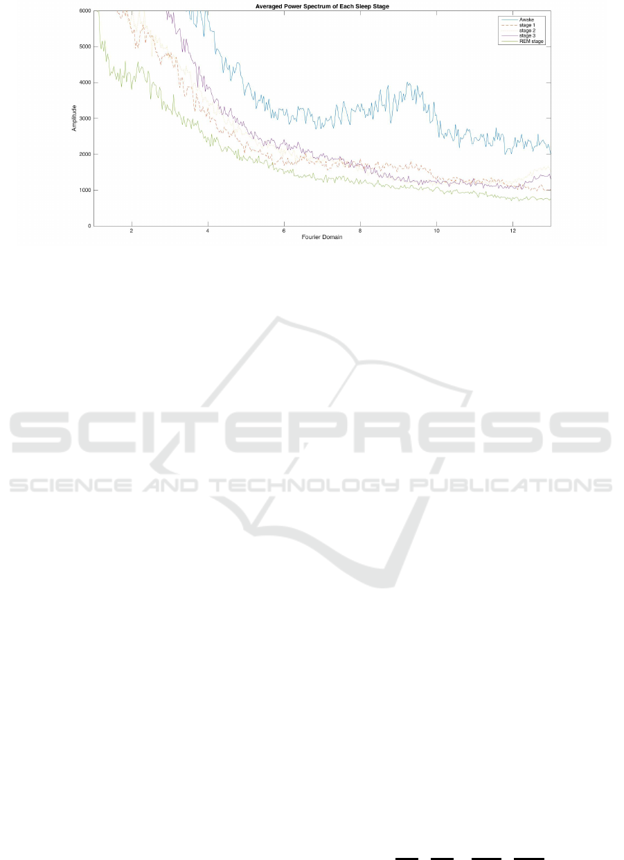
Figure 1: Averaged power spectrum of each sleep stage with the frequencies given in Hz.
The American Academy of Sleep Medicine’s manual
(Berry et al., 2012) differentiates between five stages
of sleep: Awake, Stage 1, Stage 2, Stage 3, REM
sleep, where the stages of light sleep (Stage 1 and
Stage 2) are sometimes called NREM 1 and NREM
2 (for Non-REM sleep 1 and 2) and the deep sleep
stage, Stage 3, is sometimes called NREM 3 (for Non-
REM sleep 3).
A measurement of a full night of sleep results in
approximately 960 epochs (8 hours) per patient. Fur-
ther, as recommended by AASM (Berry et al., 2012),
professional scorers rely on a full polysomnography,
which consists of several EEG nodes, EOG deriva-
tions, a Chin EMG and several other parameters for an
optimal rating of the sleep of the patient. The perfor-
mance of these measurements is not only painstaking
and expensive, but can also have a strong influence on
the sleep of the patient, leading to distorted data.
As the classification of sleep stages via profes-
sionals tends to be tedious, there have been various
approaches to automatize the procedure (Tagliazuc-
chi et al., 2012; Redmond and Heneghan, 2003; Liang
et al., 2012; Pan et al., 2012; Wang et al., 2015; An-
derer et al., 2010; Gudmundsson et al., 2005), using
methods such as SVMs, neural networks or Hidden
Markov Models. Mostly, full polysomnographic data
was used and reliabilities ranging between 70% and
90% were achieved (Penzel and Conradt, 2000); how-
ever, there has also been automatic single-channel or
two-channel sleep staging (Zibrandtsen et al., 2016;
Wang et al., 2015; Koley and Dey, 2012). In (Ko-
ley and Dey, 2012), the measurements of the elec-
trodes at the mastoid (often referred to as A
1
and A
2
or
M
1
and M
2
) were used for the classification into light
sleep, deep sleep and REM sleep, thus offering proof
that measurements at the mastoid yield enough reli-
able information for the classification into three sleep
stages. In this paper, we would like to take it one step
further by classifying into five different sleep stages,
as is usual in sleep medicine. This task proves to be
highly difficult, since the transitional stage 1 is often
uncertainly classified and can easily be mistaken for
the sleep stages 2 and Awake.
1.2 Overview and Notation
Our data set consists of A
1
- and A
2
- measurements
over 8 hours of sleep of several persons with a sam-
pling rate of 256Hz. This data is divided into blocks
of 30 seconds (so-called epochs), that contain 256 ·
30 = 7680 measurements each for A
1
and A
2
:
E
k
=

E
A
k
1
, . . . , E
A
k
T

⊆ R
7680
, T ≈ 960, k = 1, 2.
For each patient, we divide the set of epochs into a
training set and a test set
E = E
train
∪ E
test
,
E
train
=
[
k=1,2
(E
A
k
1
, . . . , E
A
k
T
train
),
E
test
=
[
k=1,2
(E
A
k
T
train
+1
, . . . , E
A
k
T
),
In our case, we divided the 8-hour-measurement into
two halves and used the first half as the training set
(which equates to T
test
≈ 480) and the second half as
the test set. This choice shall be improved in the next
stages of this project, as it is known that REM sleep
typically occurs more often in the second half of the
night. The sequence of sleep stages corresponding to
these epochs will be denoted by random variables
C = (C
1
, . . . , C
T
train
| {z }
=: C
train
, C
T
train
+1
, . . . , C
T
| {z }
=: C
test
) ∈ S
T
,
Heuristic Approximation of the MAP Estimator for Automatic Two-channel Sleep Staging
237

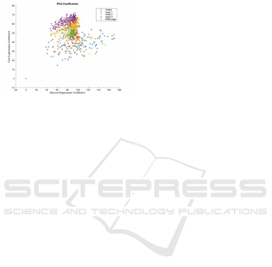
Figure 2: PCA Coefficients of the first two dominant eigen-
vectors of measurements of different sleep stages.
where the state space S consists of the five sleep
stages:
S = {’Awake’, ’Stage 1’, ’Stage 2’, ’Stage 3’, ’REM’}.
We will assume its classification by a professional
scorer (who had access to the full polysomnography),
(C
train
, C
test
)
!
= (c
prof
train
, c
prof
test
)
to be correct. Our aim is to implement an algorithm
A, that classifies the test set E
test
using only the pro-
fessional classification c
prof
train
of the training set E
train
,
A : (E
train
, E
test
, c
prof
train
) 7→ c
algo
test
∈ S
T −T
train
,
such that c
algo
test
= c
prof
test
in many components with high
probability.
2 THE ALGORITHM
2.1 Preprocessing
The frequencies in a measurement play a central role
in the classification of sleep stages (Berry et al., 2012;
Penzel and Conradt, 2000). Signals of certain fre-
quencies indicate conscious behaviour (such as the
highly-frequent beta waves) or unconsciousness (such
as delta waves). Therefore, it is meaningful to utilize
the power spectrum of a measurement. As it can be
seen in Figure 1, the average power spectra of differ-
ent sleep stages behave visibly different, except for
sleep stages one and two, which are not easily dis-
tinguishable. Furthermore, the power spectra of mea-
surements E
A
k
i
∈ R
7680
of epochs might be easier to
compare, since they are invariant under shifts in time.
Additionally, it is known that certain confounding
measurements may hinder the classification of sleep
stages. These signals, which are called artifacts, can
be caused for example by sweat on the skin of the
proband or movements of body parts, eyes etc.. How-
ever, it is also known that these artifacts typically
evoke signals that have different frequencies than the
signals, which are used for the classification of sleep
stages. Through a low pass filter, we ignore all the fre-
quencies above a fixed threshold (approximately 66
Hertz). We do so in the following manner:
E
A
k
t
∈ R
7680
7→ F
A
k
t
= |FFT(E
A
k
t
)| ∈ R
7680
.
and
F
A
k
t
7→
˜
F
A
k
t
= proj(F
A
k
t
) ∈ R
2000
,
where proj(·) is the projection of a vector onto its first
2000 coordinates. We assume this to be adequate, as
the signals used for professional scoring range in the
same frequency interval and it is known that artifacts
created by bodily movement typically involve high-
frequent signals.
We would like to remark that we have purposely
not filtered out all of the frequencies that are not used
in traditional sleep-staging in an attempt to retain as
much information as possible while still removing ar-
tifacts.
To further reduce the dimension of the data and
to make the data usable for classification, we used a
principal component analysis (PCA), where we pro-
jected the data onto the space spanned by the 15 dom-
inant eigenvectors of the covariance matrix. As it can
be seen in Figure 2, the procedure retains a consid-
erable amount of information from the measurements
and the differences of the sleep stages can be seen
even when using only the first two dominant eigen-
vectors. A scree plot was used to determine the opti-
mal amount of eigenspaces, which was 15 in our case.
To avoid an a priori bias towards the lower fre-
quencies, the Fourier transformed data is logarith-
mized before applying the PCA. This makes sense as
higher frequencies tend to have smaller amplitudes.
Let
M
k
t
= log
˜
F
A
k
t
be the logarithmized projection of the power spectrum
for a t ∈ {1, . . . , T }. We used the data matrix (M
1
t
, M
2
t
)
for the PCA
(
˜
F
A
k
t
,
˜
F
A
k
t
)
log
7−→ (M
1
t
, M
2
t
)
PCA
7−−→ m
t
∈ R
15
,
where m
t
is the projected data resulting from the PCA.
This leads to the following overall preprocessing steps
(R
7680
)
2
−→ (R
2000
)
2
−→ (R
2000
)
2
−→ R
15
(E
A
k
t
)
k
FFT
7−−→
proj
(
˜
F
A
k
t
)
k
log
7−→ (M
k
t
)
k
PCA
7−−→ m
t
.
BIOSIGNALS 2017 - 10th International Conference on Bio-inspired Systems and Signal Processing
238

We then define
X
train
:= {m
1
, . . . , m
T
train
}
X
test
:= {m
T
train
+1
, . . . , m
T
}
2.2 Hidden Markov Model and the
MAP Estimator
We assume the sequence of sleep stages C =
(C
1
, ..., C
T
) ∈ S
T
introduced in Section 1.2 to be a
Markov chain with transition matrix P ∈ R
5×5
, which
will be approximated by the empirical probabilities of
all possible transitions
P
s,s
0
=
#{x
t+1
= s, x
t
= s
0
| t = 1, . . . , T
train
− 1}
#{x
t
= s
0
| t = 1, . . . , T
train
− 1}
for s, s
0
∈ S (it is thereby not considered part of the in-
ference process). Accordingly, the invariant measure
π of the Markov chain will be approximated by the
empirical probabilities
π(s) =
#{x
τ
= s | τ = 1, . . . , T
train
}
T
train
, s ∈ S .
For the inference process, our prior konwledge
P(C
test
) about C
test
is therefore modeled by Markov
chain of length T
test
= T − T
train
with P(C
t
) = π for
each t = T
train
+ 1, . . . , T and transition matrix P .
Bayes’ rule is the proper tool to update our knowl-
edge about C
test
given the measurements X
test
:
P(C
test
| X
test
) =
P(X
test
| C
test
)P(C
test
)
P(X
test
)
.
We will mainly focus on estimating the maximum a
posteriori (MAP) estimator of C
test
,
c
MAP
test
= argmax
c
P(C
test
= c | X
test
)
= argmax
c
P(X
test
| C
test
= c)P(C
test
= c).
Since each measurement X
t
is assumed to depend only
on C
t
, we assume that all measurements
X
t
| C
test
= X
t
| C
t
, t = T
train
+ 1, . . . , T,
are independent. Therefore, the likelihood model
P(X
test
| C
test
) is be given by the product of the in-
dividual likelihoods P(X
t
| C
t
),
P(X
test
| C
test
) =
T
∏
t=T
train
+1
P(X
t
| C
t
)
the latter being trained by a pre-installed MATLAB
classifier. Theoretically, we now have all the neces-
sary ingredients to compute the MAP estimator.
2.3 Heuristic Approximation of the
MAP Estimator
Though we are now able to compute the probability
of each realization C
test
= c ∈ S
T
test
given the mea-
surements X
test
, the straightforward approach of com-
puting all these probabilities is impractical due to the
huge number of possible chains,


S
T
test


= 5
T
test
≈ 3 · 10
335
.
Therefore, a heuristic approach is necessary in order
to compute these probabilities P(C
test
= c | X
test
) only
for “realistic” or “probable” chains. Since we are
only interested in the MAP estimator c
MAP
test
and not
in the whole probability distribution of C
test
|X
test
, this
restriction is meaningful, however, it will only yield
an approximation of c
MAP
test
.
For the heuristic approach let us first introduce the
notation
C
t
:= (C
t
Train
+1
, . . . , C
t
Train
+t
),
X
t
:= (X
t
Train
+1
, . . . , X
t
Train
+t
),
π
t
(c
t
) := P(X
t
| C
t
= c
t
)P(C
t
= c
t
),
the latter being the value we want to maximize for
t = T
test
.
We will proceed as follows:
1. Compute all possible (5
4
= 625) values of π
4
.
2. For t = 5, . . . , T
test
, iterate
(a) Restrict the set of considered subchains
(c
1
, . . . , c
t−1
) to 125 subchains with the highest
values of π
t−1
.
(b) Compute π
t
for all possible subchains
(c
1
, . . . , c
t
) that contain the above subchains
(5 · 125 = 625 values).
This way, chains with unlikely subchains are dis-
carded successively and we end up with 625 very
probable (but possibly not most probable) chains.
Step (b) in the above iteration can be performed very
efficiently via the formula
P(C
t
| X
t
) ∝ P(C
t−1
| X
t−1
)P(C
t
| C
t−1
)P(X
t
| C
t
).
Through this heuristic, the number of evaluations of
this formula is reduced to 125 in each timestep.
3 RESULTS
The method was tested on five healthy subjects at
the sleep laboratory of the Advanced Sleep Research
GmbH. Each patient’s sleep was measured with a full
polysomnography for a duration of approximately 8
Heuristic Approximation of the MAP Estimator for Automatic Two-channel Sleep Staging
239

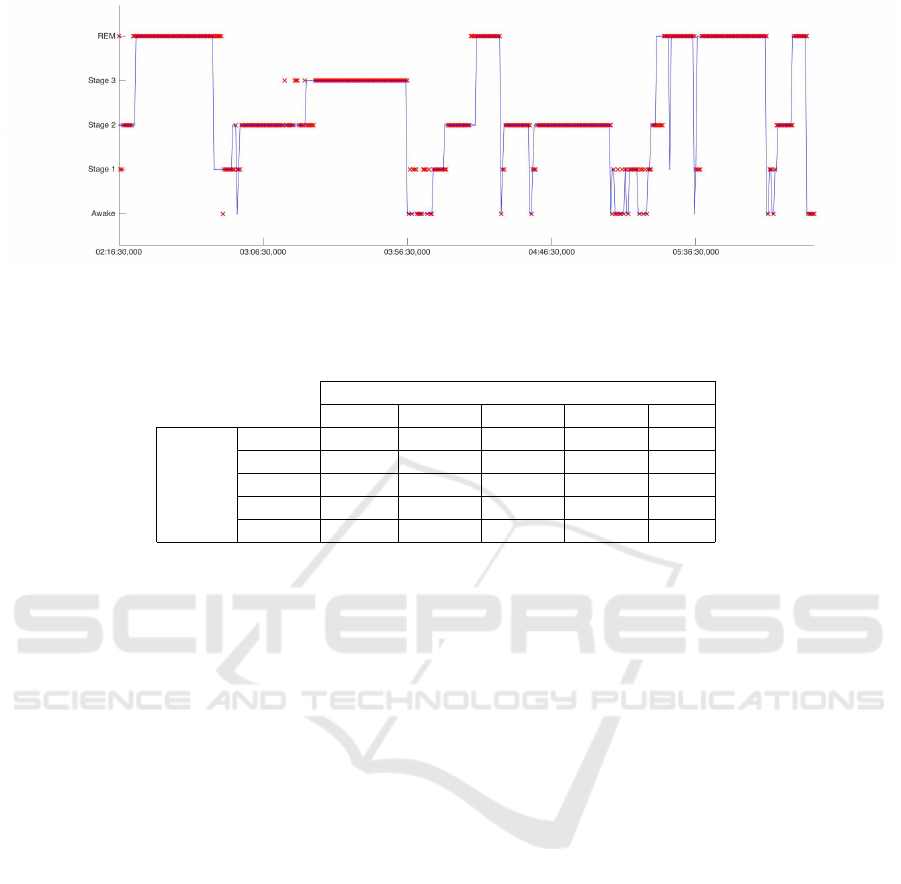
Figure 3: Sleep stage classification of the second half of the measurement. Comparison of the MAP estimator method (blue)
and the classification of a professional scorer (red).
Table 1: Confusion matrix of patient 3, where the classifications of a professional scorer are compared to the output of the
algorithm.
Classification
Awake Stage 1 Stage 2 Stage 3 REM
Stages Awake 27 2 0 0 0
Stage 1 17 31 11 0 3
Stage 2 2 1 145 6 6
Stage 3 1 0 5 64 0
REM 3 7 7 0 145
hours. As stated before, the first half of the night was
used as training data, whereas the second half of the
night was used to test the algorithm. The hypnogram
that was used as the “ground truth” to train and verify
the algorithm was scored by a professional somnolo-
gist, who used a full polysomnography.
The error rates for the five subjects were 14%,
24%, 34%, 22% and 31%, respectively. Thus, they
are ranging between 14%-34% with an average of
25%.
As one can see in Figure 3, the overall structure of
the classification of the algorithm is very close to the
scoring of a professional, who had the advantange of
using a full polysomnography.
The evaluation of the confusion matrices showed
that the classification of the Awake stage, as well as
stages 2 and 3 are fairly adequate. Stage 1 is often
mistaken for the Awake stage or stage 2 and REM
stage is sometimes mistaken for one of the light sleep
stages, as it can be seen in Table 1.
4 DISCUSSION
Summing things up, we can conclude that the mea-
surements at A
1
and A
2
contain relevant information
for automatic sleep-scoring. This can be viewed as a
proof of concept, as these positions are usually only
used as reference electrodes. Beyond the recognition
of wakefulness and sleep, the MAP estimator offers
differentiated classifications.
It appears that, in contrast to earlier methods used
for the classification of sleep stages, the method pre-
sented in this paper seems to prefer continuous struc-
tures. Especially in phases of transition between
stages, where professional scorers seem to be uncer-
tain, the MAP estimation method prefers a single tran-
sition in contrast to the erratic behaviour of the pro-
fessional scorer.
It could be argued that such an undecisive phase
between the stages should be flattened with respect to
the preceding and the following sleep stage. In this
case, it is unclear, whether classification of the auto-
matic method or the scorer is preferable.
Usually, patients are requested to spend two nights
at a sleep laboratory, in order to minimize confound-
ing effects. A minimized measurement system with
the patient-specific algorithm at hand could replace
the second measurement and thus halve the costs for
sleep-related diagnosis at worst. At best, the algo-
rithm could learn to transfer the classification from
one person to another.
ACKNOWLEDGEMENTS
We would like to thank the Charit
´
e Universit
¨
atsmedi-
zin Berlin as well as the Advanced Sleep Research
GmbH for providing the data for testing the method.
BIOSIGNALS 2017 - 10th International Conference on Bio-inspired Systems and Signal Processing
240

REFERENCES
Anderer, P., Moreau, A., Woertz, M., Ross, M., Gruber,
G., Parapatics, S., Loretz, E., Heller, E., Schmidt, A.,
Boeck, M., et al. (2010). Computer-assisted sleep
classification according to the standard of the amer-
ican academy of sleep medicine: validation study of
the aasm version of the somnolyzer 24× 7. Neuropsy-
chobiology, 62(4):250–264.
Berry, R. B., Brooks, R., Gamaldo, C. E., Harding, S. M.,
Marcus, C., and Vaughn, B. (2012). The aasm manual
for the scoring of sleep and associated events. Rules,
Terminology and Technical Specifications, Darien,
Illinois, American Academy of Sleep Medicine.
Gudmundsson, S., Runarsson, T. P., and Sigurdsson, S.
(2005). Automatic sleep staging using support vec-
tor machines with posterior probability estimates.
In International Conference on Computational In-
telligence for Modelling, Control and Automation
and International Conference on Intelligent Agents,
Web Technologies and Internet Commerce (CIMCA-
IAWTIC’06), volume 2, pages 366–372. IEEE.
Kales, A., Rechtschaffen, A., University of California,
L. A., and (U.S.), N. N. I. N. (1968). A manual of stan-
dardized terminology, techniques and scoring system
for sleep stages of human subjects. Allan Rechtschaf-
fen and Anthony Kales, editors. U. S. National Insti-
tute of Neurological Diseases and Blindness, Neuro-
logical Information Network Bethesda, Md.
Koley, B. and Dey, D. (2012). An ensemble system for
automatic sleep stage classification using single chan-
nel eeg signal. Computers in biology and medicine,
42(12):1186–1195.
Liang, S.-F., Kuo, C.-E., Hu, Y.-H., and Cheng, Y.-S.
(2012). A rule-based automatic sleep staging method.
Journal of neuroscience methods, 205(1):169–176.
Pan, S.-T., Kuo, C.-E., Zeng, J.-H., and Liang, S.-F.
(2012). A transition-constrained discrete hidden
markov model for automatic sleep staging. Biomed-
ical engineering online, 11(1):1.
Penzel, T. and Conradt, R. (2000). Computer based
sleep recording and analysis. Sleep medicine reviews,
4(2):131–148.
Redmond, S. and Heneghan, C. (2003). Electrocardiogram-
based automatic sleep staging in sleep disordered
breathing. In Computers in Cardiology, 2003, pages
609–612. IEEE.
Tagliazucchi, E., von Wegner, F., Morzelewski, A., Borisov,
S., Jahnke, K., and Laufs, H. (2012). Automatic sleep
staging using fmri functional connectivity data. Neu-
roimage, 63(1):63–72.
Wang, Y., Loparo, K. A., Kelly, M. R., and Kaplan, R. F.
(2015). Evaluation of an automated single-channel
sleep staging algorithm. Nature and science of sleep,
7:101.
Zibrandtsen, I., Kidmose, P., Otto, M., Ibsen, J., and Kjaer,
T. (2016). Case comparison of sleep features from
ear-eeg and scalp-eeg. Sleep Science.
Heuristic Approximation of the MAP Estimator for Automatic Two-channel Sleep Staging
241