
Training Agents with Neural Networks in Systems with Imperfect
Information
Yulia Korukhova and Sergey Kuryshev
Computational Mathematics and Cybernetics Faculty, M.V. Lomonosov Moscow State University,
Leninskie Gory, GSP-1, Moscow, 119991, Russian Federation
Keywords: Multi-agent Systems, Neural Networks, Dominated Strategies.
Abstract: The paper deals with multi-agent system that represents trading agents acting in the environment with
imperfect information. Fictitious play algorithm, first proposed by Brown in 1951, is a popular theoretical
model of training agents. However, it is not applicable to larger systems with imperfect information due to
its computational complexity. In this paper we propose a modification of the algorithm. We use neural
networks for fast approximate calculation of the best responses. An important feature of the algorithm is the
absence of agent’s a priori knowledge about the system. Agents’ learning goes through trial and error with
winning actions being reinforced and entered into the training set and losing actions being cut from the
strategy. The proposed algorithm has been used in a small game with imperfect information. And the ability
of the algorithm to remove iteratively dominated strategies of agents' behavior has been demonstrated.
1 INTRODUCTION
In any complex multi-agent system the optimal
behavior of each agent depends on the behavior of
other agents. A key feature of agents is the ability to
learn and adapt to the conditions of an unfamiliar
environment. Therefore, games with imperfect
information represent a good platform for testing the
behavior of agents’ algorithms. Current state-of-art
approaches to finding optimal strategies for games
with imperfect information, such as CFR (Zinkevich
et al., 2007, Gibson, 2014) or linear programming
(Koller et al., 1994), are based on a priori knowledge
about the game, and do not fully reflect the learning
process of agents. In this paper we propose a
learning algorithm for agents without built-in
information about the environment. It is based on the
algorithm of fictitious play (Brown, 1951), and
allows to overcome some of its limitations. The
classic version of Brown's algorithm requires the
calculation of the exact best responses at each step
which is computationally challenging. The proposed
modification replaces the calculation of the exact
best responses at each step with the calculation of
the approximate best responses by neural networks.
At the same time agents initially have no knowledge
about the environment, and obtain it during
interaction by encouraging actions that lead to
success and cutting losing actions.
We begin with the definition of extensional
forms games which represent a good framework for
the description of multi-agent systems, and describe
some concepts of game theory. Then we will briefly
describe fictitious play algorithm and its limitations.
After that, we will present our algorithm and
demonstrate its ability to avoid iteratively dominated
strategies on the example of Kuhn poker - simple
game with imperfect information (Kuhn, 1950).
2 BACKGROUND
2.1 Extensive-form Games
Extensive-form game representation is widely used
to describe sequential systems with imperfect
information and stochastic events. It can be viewed
as a directed tree, where each non-terminal node
represents a decision point for an agent and each leaf
of the tree corresponds to winnings for the selected
sequence of actions. If game includes stochastic
events, such as a dice roll or dealing of cards, it is
simulated by adding a special chance agent with a
fixed strategy according to probabilities of stochastic
296
Korukhova Y. and Kuryshev S.
Training Agents with Neural Networks in Systems with Imperfect Information.
DOI: 10.5220/0006242102960301
In Proceedings of the 9th International Conference on Agents and Artificial Intelligence (ICAART 2017), pages 296-301
ISBN: 978-989-758-219-6
Copyright
c
2017 by SCITEPRESS – Science and Technology Publications, Lda. All rights reserved
events. In games with imperfect information tree
nodes for each agent are combined into the so-called
information sets so that the agent cannot distinguish
between such nodes within one set based on the
information available to him.
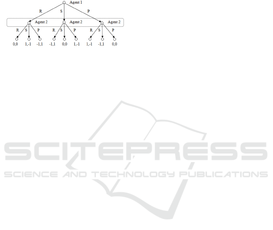
Figure 1: The game of "rock, paper, scissors" in the
extensive form.
Figure 1 shows the extensive form of the "rock,
paper, scissors" game. Since decisions are made
simultaneously, agent 2 cannot distinguish between
states, dashed circled, and he must have the same
strategy in all of those nodes. These nodes form the
information set for agent 2.
Here is the formal definition of extensive form
games with imperfect information:
Definition 1 (Osborne and Rubinstein, 1994). The
game of imperfect information in the extensive form
is a tuple (,,,
,,), where
• N - a finite set of players
• H – a set of sequences satisfying the following
conditions:
o An empty sequence ∅ is contained in H.
o If the sequence (
)
,…,
∈and <
, then any subsequence.(
)
,…,
∈
o If an infinite sequence (
)
satisfies the
condition ∀ ∈ (
)
,…,
∈, then
(
)
∈
(Each member of the sequence is called the
history; each component of the history is an
action for the player). The history
(
)
,…,
∈
is terminal, if it is infinite, or if there is no
such that
(
)
,…,
∈.
(
)
:
(
,
)
∈
is the set of actions
available after the nonterminal history . The set
of terminal histories is denoted by .
• - a function that assigns an element of the set
∪ to each nonterminal history. (() is
called the player's function and shows whose
turn to act after the history . If () , an
action after the history is determined by
chance.)
•
- a function that assigns to each nonterminal
history , for which () , a probability
measure
(
∙
|
)
on (), where each such
probability measure is independent of the
others. (
(
|
)
is the probability that the
action will be taken after a history )
• For each player ∈
:→ is an utility
function that determines the winnings for player
for each terminal history ∈.
• For each player is ∈
is a partition
∈ :
(
)
, so that
(
)
(
)
if
and ′ belongs to the same partition member.
For
∈
(
)
defines the set of (),
(
)
defines a player P(h) for any history ∈
.
(
- is a information partition for the player ;
∈
– information set for player )
Definition 2. Pure strategy of player ∈ in an
extensive form game with imperfect information is a
function that assigns an action from
(
)
to each
information set
∈
.
There are two ways of modeling possibilities of
the players randomly select actions in certain states
in extensive form-games.
Definition 3. Mixed strategy for player in the
extensive form game is a probability distribution
over the set of pure strategies of the player.
Definition 4. Behavioral strategy for player is a set
of independent probability measures (
(
)
)
∈
,
where
(
)
is a probability distribution over
(
)
.
The difference in the two definitions
reflects two possible random choices of the player's
actions: he can randomly select a pure strategy
before the start of the game, or he can randomly
choose the action each time during his turn. The
most common concept of solving games is Nash
equilibrium.
Definition 5. Nash equilibrium (Nash, 1951) is a
strategy profile where none of the players can
increase his winnings by changing his strategy
unilaterally:
(
,
)
:
(
)
max
′
∈Σ
(
′
,
)
(
)
max
′
∈Σ
(
,
′
)
In large games it is often not possible to calculate
the exact Nash equilibrium. Instead one can
calculate it’s approximation.
Definition 6. -nash equilibrium is strategy profile
where none of the players can increase his winnings
by more than changing his strategy unilaterally:
(
,
)
:
(
)
+max
′
∈Σ
(
′
,
)
(
)
+max
′
∈Σ
(
,
′
)
In competitive games equilibrium strategies are so
Training Agents with Neural Networks in Systems with Imperfect Information
297

complex that most of the players deviate from them
in any way. A good player should notice and exploit
such deviations to increase his own gain. In this
case, the applicable concept is the best response.
Let
be the profile of strategies of player’s
opponents - all strategies from profile except
.
Then the best response for player to opponents’
profile
will be
∗
∈
(
,
).
In the case of Nash equilibrium strategies of the
players are the best responses to each other.
Definition 7. A player's strategy
is weakly
dominated if there is a different strategy for this
player
′
, such that
1)
(
,
)
≤
′
,
∀
∈ Σ
,
2) ∃
∶
(
,
)
<
′
,
If the second condition is satisfied for all the profiles
of opponents’ strategies
∈ Σ
, a strategy is
called strictly dominated.
For each type of domination iteratively dominated
strategy can be defined recursively as any strategy
that is dominated at present, or becomes dominated
after excluding iteratively dominated strategies from
the game.
2.2 Poker
Poker is a class of card games with two or more
players. There are more than 100 poker variants with
different rules. General elements of all types of
poker are completely or partially closed opponents’
cards, card combinations, and the presence of trade
during the game. Poker has interesting properties
that cannot be analyzed by conventional approaches
used in games with the full information:
• Incomplete information about the current
state of the game. In most variants of poker
players cannot see opponent's cards.
• Incomplete information about opponents’
strategy. The hidden information is not always
revealed to players at the end of the game,
which is an obstacle to the definition of
strategies of opponents. Therefore, opponents
have to use simulation approaches based on the
frequency of their actions.
• Stochastic events. The random distribution of
cards makes the players to take risks.
• Various numbers of players (2 to 10). Games
with more than one opponent are strategically
different from the games of two players, as the
Nash equilibrium is not giving a break-even
guarantees. Opponents may accidentally or
deliberately choose a strategy so that a player’s
strategy from equilibrium profile will lose.
• Repeated interaction. Poker is a series of short
games or hands, where after each hand the
player receives partial information about his
opponent, which allows him to make
adjustments in their strategy.
• Importance of opponents’ errors
exploitation.
2.2.1 Kuhn Poker
Even the smallest variant of competitively played
poker has a large number of game states (Johanson,
2013), and the game requires a lot of computing
power to solve. So much smaller variations of poker,
retaining its basic properties, are often applied for
testing algorithms.
Kuhn poker was proposed by Harold Kuhn in
1950. It is a very simple version of poker, which is
attended by two players. The deck consists of three
cards: queen, king and ace, the game takes place
only one round of bidding, and only 4 actions are
available to players: bet, check, call and fold. The
game is played as follows:
• Both players initially make a bet of 1 chip into
the pot, called the ante.
• Each player is dealt one card
• The first player can choose to bet or check.
The amount of betting is fixed to 1 chip.
• If the first player selects a bet, the second player
can play call, or fold
o In the case of call the showdown
occurs. The player with the highest
card wins the pot.
o In the case of fold the pot goes to the
first player.
• If the first player chooses a check, the second
player can play a bet or a check
o If the second player selects the check
the showdown occurs. The player with
the highest card wins the pot.
o If the second player selects the bet, the
first player can play call, or fold
In the case of call the showdown
occurs. The player with the
highest card wins the pot.
In the case of folding pot goes to
the second player.
Kuhn poker can be generalized to multiple
players version. In this case, a deck for players
will consist of +1 cards. Kuhn poker with three
players is used as one of the games at the Annual
Computer Poker Championship.
ICAART 2017 - 9th International Conference on Agents and Artificial Intelligence
298
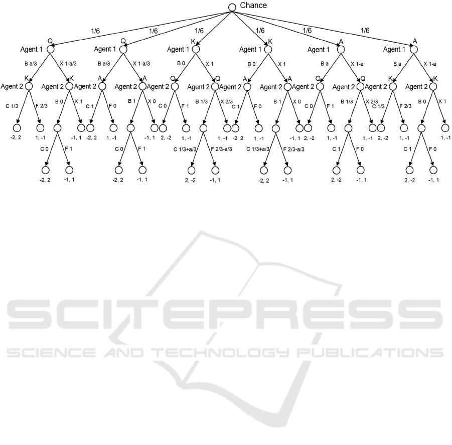
Figure 2: Nash equilibrium in Kuhn poker.
Kuhn poker is fairly simple so Nash equilibrium
(fugure 2) and dominated strategies can be
calculated manually in the case of two players.
Dominated strategies in Kuhn poker are
strategies containing the following actions with
more than 0 probability:
• Fold with the ace by second player after first
player’s bet. When the second player has the
ace, the first player may only have a king or
queen, and thus calling a bet will lead the first
player to winning 2 chips, while folding to the
loss of one chip.
• Call with the queen be second player after
first player’s bet. Similarly, calling a bet with
the queen, when the enemy is always has better
card leads to losing more compared to fold.
• Check with the ace by second player after
first player’s check. Checking with ace leads to
a gain of 1 chip, while betting in the worst case
(when the enemy always folds) leads to a gain
of 1 chip. If the opponent at least sometimes
makes a call, the gain becomes greater than 1
chip.
• Fold with the ace by first player after second
player’s bet. The proof is similar to the first
paragraph.
• Call with the queen by first player after
second player’s bet. The proof is similar to the
second paragraph.
All the above examples are parts of weakly-
dominated strategies, as the enemy might choose a
strategy that does not generate required sequences of
actions. And this will lead to unstrict inequality in
definition 5.
After the removal of the strategies described
above, strategies containing the following parts
becomes dominated:
• Bet with the king by second player. The
enemy always folds with queen and calls with
ace. Thus, the average gain after bet is -0.5
chips. Average gain after check is 0.
• Bet with the king by first player. The proof is
similar.
It is easy to show that there are no any dominated
strategies left in Kuhn poker. Kuhn poker has an
infinite number of Nash equilibrium profiles, where
the strategy of the first player is determined by the
parameter , and the second player's strategy is
constant.
3 TRAINING AGENTS WITH
NEURAL NETWORKS
In this paper we consider multi-agent system that
represents trading agents acting in the environment
with imperfect information. The essence of the
fictitious play (FP) algorithm is that the agents
repeatedly play the game, selecting the best counter-
strategy to the average opponents’ strategies on each
iteration. In this case average strategy profile
converges to Nash equilibrium in certain classes of
games, in particular in zero-sum game. However,
this approach has not found widespread use in large
games due to its dependence on the representation of
the game in the normal form and poor scalability.
Training Agents with Neural Networks in Systems with Imperfect Information
299
We propose a modification of FP algorithm using
neural networks to build strategies for multi-agent
systems. In our approach agent’s strategy is stored as
a neural network. Network’s input is the current
state of the game. Network’s output is a probability
distribution over all possible actions in the current
state. The advantage of this approach, as compared
to conventional methods of constructing strategies in
multi-agent systems is the lack of built-in
information about the environment, and as a result
its versatility. The pseudo-code of the algorithm is
shown below.
InitAgent (arbitrary);
for (i = 1; i <numSteps; i ++) {
handHistory = Play(Agent, Agent,
numHands);
foreach(actHistory) {
hhByAaction[actHistory] =
CutHH(handHistory,actHistory);
SortByEV(hhByAaction);
for (j = 1; j<length
(hhByAaction[actHistory])
/learningRate;
j++) {
action = CutAction(
hhByAaction[actHistory][j]);
AddToTrainInput(actHistory);
AddToTrainOutput(action);
}
}
Agent.neuralNet = train
(Agent.neuralNet, trainInput,
trainOutput);
}
Code 1: Agent’s learning algorithm.
First the agent’s neural network is initialized so
that it outputs equal probabilities of actions on each
game state. An important difference between this
initialization from the random one is that it allows
the agent to try different actions on the first step of
the algorithm. While the neural network, resulting
from random initialization can have zero or very low
probabilities of certain actions, and thus the agent
will never know how good or bad it is.
At each step of the algorithm agent plays himself
numHands hands and saves the hand history. Then
this history is divided into sub-histories according to
states of the game. Each sub history is sorted by
winnings for the relevant agent. A certain number of
sub-history’s first elements are added to the training
set, depending on the learning rate. Then agent trains
his neural network. Thus, the strategy at each step is
replaced by the approximate best response to the
previous agent’s strategy.
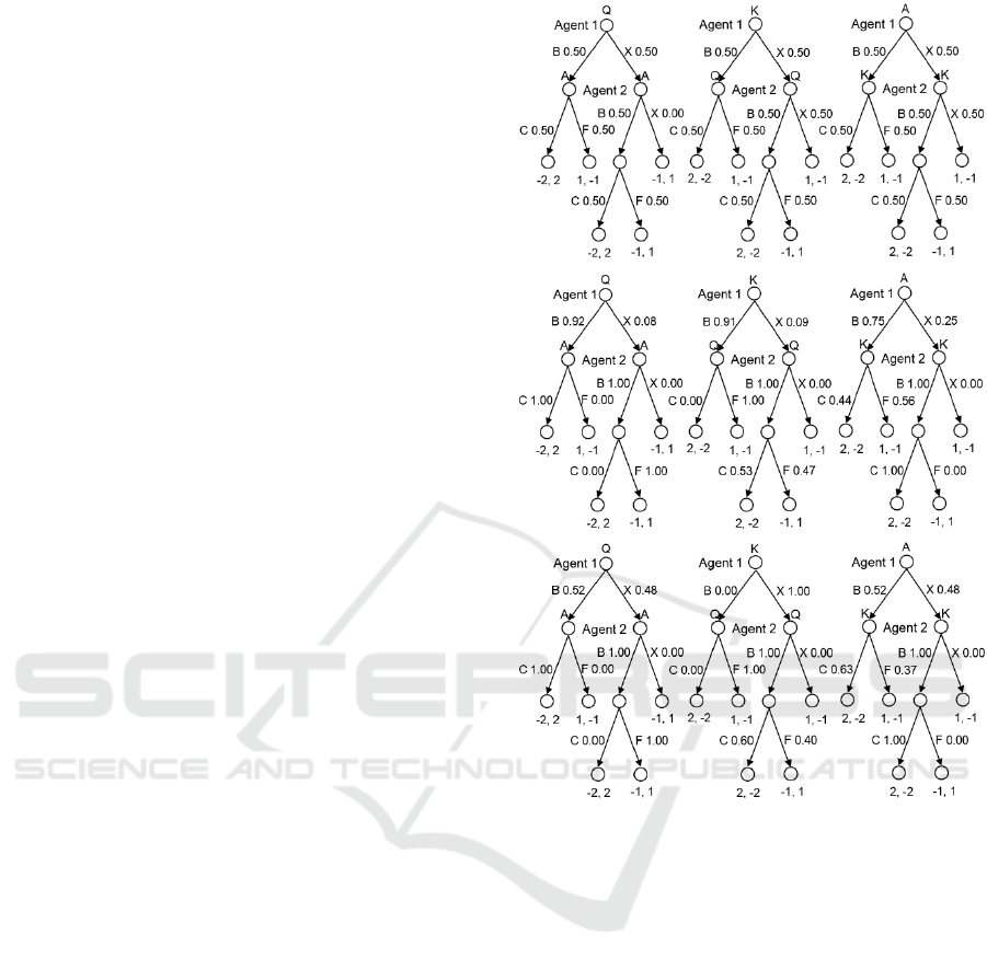
Figure 3: The results of the algorithm for QA, KQ and AK
subtrees on the 1st, 2nd and 10th step.
The algorithm was implemented in MATLAB and
tested on Kuhn poker. Kuhn poker has a small
number of game states, but retains all the key
features of games with imperfect information. Nash
equilibrium and dominated strategies in Kuhn poker
can be calculated manually, which is convenient for
the evaluation of the program. The following
parameters were used in the testing algorithm
training agents in Kuhn poker:
numSteps = 10, numHands = 100, learningRate = 5.
The results of the program by steps for QA, KQ and
QK subtrees are shown on the figure 3.
Since agents can’t distinguish game states where
their opponents have different hole cards using these
subtrees is enough to show full agent’s strategy
It can be seen that a part of the dominated
strategies has been removed. But on the second step
of the algorithm agent’s 2 bet with every card after
agent’s 1 check became approximate best response.
ICAART 2017 - 9th International Conference on Agents and Artificial Intelligence
300

After the agent’s strategy was changed to this
approximate best response, the agent stopped to
select check in this state, and thereby lost the
opportunity to learn that the check may be better
than bet. To resolve this problem, an algorithm has
been modified, and the strategy of the agent at each
step was replaced not with approximate best
response:
Agent.neuralNet =
train(Agent.neuralNet, trainInput,
trainOutput);
but with the arithmetic mean of best response and
previous strategy:
Agent.neuralNet = (Agent.neuralNet +
train (Agent.neuralNet,trainInput,
trainOutput)) / 2;
The results of the modified algorithm on the 10
th
step are shown on the figure 4.
Figure 4: The results of modified algorithm on the 10
th
step.
The modified algorithm removed all iteratively
dominated strategies from the game. The best
response accuracy and thus convergence to Nash
equilibrium depends heavily on the method of
generating training set for the neural network on
each step. We will continue our work to reach and
prove the convergence of the algorithm to Nash
equilibrium.
4 CONCLUSIONS
In this paper an algorithm for training agents in
imperfect information systems with neural networks
was proposed. An important feature of the algorithm
is the absence of a priori knowledge of the system.
Agents’ learning goes through trial and error:
winning actions are encouraged and stored into the
training set, losing actions are cut from the strategy.
The proposed algorithm has been tested on a small
game with imperfect information and its ability to
remove iteratively dominated strategies of agents'
behavior has been demonstrated. However, further
research is required to ensure the convergence of the
strategy profile to Nash equilibrium.
REFERENCES
Nash, J. 1951. Non-cooperative games. The Annals of
Mathematics, Second Series, Volume 54, Issue 2,
pp. 286-295.
Kuhn, H.W., 1950. Simplified Two-Person Poker. In
Kuhn, H.W.; Tucker, A.W. Contributions to the
Theory of Games 1. Princeton University Press. pp.
97-103.
Brown, G.W., 1951. Iterative Solutions of Games by
Fictitious Play. In Activity Analysis of Production and
Allocation, TC Koopmans (Ed.), New York: Wiley.
Gibson, R., 2014. Regret Minimization in Games and the
Development of Champion Multiplayer Computer
Poker-Playing Agents. Ph.D. Dissertation, University
of Alberta, Dept. of Computing Science.
Johanson, M., 2013. Measuring the Size of Large No-
Limit Poker Games. Technical Report TR13-01,
Department of Computing Science, University of
Alberta.
Zinkevich, M., Johanson, M., Bowling, M., Piccione,C.,
2007. Regret Minimization in Games with Incomplete
Information. Advances in Neural Information
Processing Systems 20 (NIPS).
Osborne M.J., Rubinstein A., 1994. A course in game
theory. MIT Press.
Koller, D., Megiddo, N. and von Stengel, B., 1994. Fast
algorithms for finding randomized strategies in game
trees. Proceedings of the 26
th
CAN Symposium on the
Theory of Computing, pp. 750-759.
Training Agents with Neural Networks in Systems with Imperfect Information
301
