
A Neuro-automata Decision Support System
for Phytosanitary Control of Late Blight
Gizelle Kupac Vianna, Gustavo Sucupira Oliveira and Gabriel Vargas Cunha
Departamento de Matematica, Universidade Federal Rural do Rio de Janeiro, BR-465, Km 7, 23897-000, Seropedica, RJ, Brazil
Keywords: Decision Support System, Cellular Automata, Pattern Recognition, Artificial Neural Networks, Digital
Images Processing.
Abstract: Foliage diseases in plants can cause a reduction in both quality and quantity of agricultural production. In
our work, we designed and implemented a decision support system that may small tomatoes producers in
monitoring their crops by automatically detecting the symptoms of foliage diseases. We have also
investigated ways to recognize the late blight disease from the analysis of tomato digital images, using a
pair of multilayer perceptron neural network. One neural network is responsible for the identification of
healthy regions of the tomato leaf, while the other identifies the injured regions. The networks outputs are
combined to generate repainted tomato images in which the injuries on the plant are highlighted, and to
calculate the damage level at each plant. That levels are then used to construct a situation map of a farm
where a cellular automata simulates the outbreak evolution over the fields. The simulator can test different
pesticides actions, helping in the decision on when to start the spraying and in the analysis of losses and
gains of each choice of action.
1 INTRODUCTION
Over the centuries, science and technology in
agronomy have been searching ways to improve
productivity, in order to feed constantly growing
populations, meanwhile important climatic changes
affect agricultural production. An important field of
research in this area is plant pathology, since many
diseases affecting plants can cause economic, social
and ecological losses. In this context, it is very
important to have a quick and accurate diagnosis of
diseases to which a plant is susceptible.
In Brazil, where an important part of the
economy depends on agriculture, it is essential that
farmers maintain a strict control over the quality of
their crops. In 2015, the agribusiness corresponded
to 21.46% of the Brazilian GDP, or more than
US$400.00 million (IBGE, 2016; MAPA, 2016).
Particularly, the tomato (Solanum lycopersicon)
crop occupies the seventh position in the rank of
food plant tons produced per year, with more than
1.9 tons produced in 2014 (IBGE, 2016). However,
that plant is vulnerable to many diseases and
requires extreme care in terms of fertilization and
phytosanitary treatment, ranking the second position
in pesticide consumption per planted area in Brazil
(Neves et al., 2003), where tomatoes are typically
produced in small farms and require continuous
monitoring from experts, which might be
prohibitively expensive and time-consuming. Thus,
the search for fast, less expensive and accurate
methods to detect the foliage diseases is of great
significance.
Many studies show the impact of plant diseases
over the quality of agricultural products (Zamberlan
et al., 2014; Tilman et al., 2002; Rembialkowska,
2007). The most common disease that affects tomato
crops worldwide is the late blight, a very damaging
disease also widespread in Brazil. The tomato late
blight is caused by Phytophthora infestans, a fungus
that inhabits the soil and disseminates through
spores. The disease occurs especially in cold and
humid months when the dispersion of spores is
facilitated by wind and high humidity, and they
reach the leaves, fruits, and branches, where they
germinate, producing a new infection focus. The
disease can spread quickly, specially under favorable
climatic conditions consisting of a combination of
relative humidity under 90% and temperature around
20°C (68°F). As a result, we have an epidemic that
can lead to considerable losses in production
(Mizubuti et al., 2002; USDA, 2016).
Vianna, G., Oliveira, G. and Cunha, G.
A Neuro-automata Decision Support System for Phytosanitary Control of Late Blight.
DOI: 10.5220/0006236104810488
In Proceedings of the 19th International Conference on Enterprise Information Systems (ICEIS 2017) - Volume 1, pages 481-488
ISBN: 978-989-758-247-9
Copyright © 2017 by SCITEPRESS – Science and Technology Publications, Lda. All rights reserved
481

On the other hand, the indiscriminate use of
pesticides in tomato fields brings serious problems
not only to human health but also to the
environment. Moreover, pathogens have started
developing resistance to the conventionally used
fungicides and a second generation of more
expensive fungicides began to be used. Therefore, it
is critical to use fungicides in proper doses and
intervals (Saxena et al., 2014; Goufo et al., 2008;
Zhang et al., 2013; Park et al., 2014).
The goal of this paper is to present a novel
computer-based solution that may help farmers to
make better decisions to combat late blight on
tomato crops, expanding previous works (Vianna
and Cruz, 2013a; Vianna and Cruz, 2013b). This
research aims at helping the detection of late blight
in tomato crops, and the measuring of the damage
level at each plant, by using a pattern recognition
system based on multilayer perceptron neural
networks (MLP). We also developed a decision
support system that generates simulations of
spreading scenarios of contamination and tests
alternatives for combating the disease, supported by
meteorological data and prediction models of the
late blight.
2 INFORMATION
TECHNOLOGY IN
AGRICULTURE
Agriculture production systems have frequently
benefited from the incorporation of technological
advances and with the aid of information technology
for early detection of crop diseases, it was possible
to delay the beginning of pesticides spraying in
comparison with the fixed schedule spraying method
(Zhanga et al., 2002; Sankaran et al., 2010; Mahlein
et al., 2012). We can find examples in the literature
where results obtained by monitoring the spores of
tomato late blight in the air allowed producers to
obtain an average reduction of 50% in total sprays,
reaching rates of 80% reduction in some cases
(Bugiani et al., 1995).
2.1 Pattern Recognition in Diagnosis of
Tomato Diseases
Farmers and workers visually recognize the disease
by the appearance of dark brown lesions on tomato
leaves that vary from brown or grey to pale green,
often situated at the edges of the leaves (Correa et
al., 2009).
In Brazil, the most common approach used in the
fight of the disease involves naked eye observations
and manual classification of the degree of infestation
at each plant. This classification is based on a visual
comparison between the infested leaf and some
schematic images of tomato leaves that quantify the
degree of infestation in a logarithmic scale (Correa
et al., 2009). After analyzing some samples of plants
from the farm, the mean of infestation degree at each
sample is used to define a schedule of pesticide
spraying.
2.2 Digital Approaches for Analysis of
Plant Leaves
Image processing is a useful tool for analysis in
various agricultural applications and several studies
have also investigated the use of broadband color, or
chromaticity values, for plant species recognition
(Sankaran et al., 2010; Barbedo, 2013; Vibhute and
Bodhe, 2012; Bock et al, 2010). One of the key
advantages of these techniques is that pixel-based
color classifiers tend to be less computationally
intensive than shape-based methods (Nixon and
Aguado, 2008). In this paper, we used the color
tones from individual pixels of the leaves to classify
them in one of the seven possible degrees of the
scale from (Correa et al., 2009). The images were
captured directly from the field, and so it is expected
that they contain a significant amount of noise from
the background and shadows. We used a mean filter
to reduce the details of abrupt color changes, which
improved the performance of our pattern classifier.
3 MATERIAL AND METHODS
3.1 Processing of Digital Images of
Leaves
At the beginning of this research, we decided to
provide our target users with the free use of our
classification system. In addition, as they are small
farmers, they may not afford expensive equipment
or might be unable to operate it properly. Thus, we
have not used any sophisticated machinery or
proprietary software packages to lower the cost of
the final system. Based on that premise, we worked
upon digital images obtained by low-resolution
built-in cell phone cameras. The pictures were taken
in an open environment under natural sunlight
conditions in the experimental fields of the
Horticulture Department of our institution in a
ICEIS 2017 - 19th International Conference on Enterprise Information Systems
482

cropping area historically linked with the natural
occurrence of late blight.
We used a combination of two ANN’s to
perform, for each pixel, its classification into one of
three possible categories: healthy, injured or
background. After classifying all the pixels of one
single image, we used the class information of all
these pixels to compute the final classification of the
whole leaf, assigning it a degree of contamination,
as defined in (Correa et al., 2009).
In the sequence of processes performed over the
digital images, the first step was to reduce the
definition, achieving 70% of the original size, to
speed up the performance of further procedures.
After that, for each image, we generated a text file
that contained, for each pixel, the X-Y coordinates
of the pixel and its RGB and HSL values. Next, all
variables were linearly normalized, generating a new
data table containing RGB and HSL values, varying
from 0 to 1, which suits better to the training process
of an ANN. We chose that normalization technique
because the variable scales are similar (R,G, and B
varies from 0 to 255; H vary from 0 to 359; S and L
varies from 0 to 100) and because, as the domain is
limited, there is no possibility of occurring outliers.
3.2 Pattern Recognition System
We conducted an experiment using two different
ANNs. The first ANN was trained to recognize
green tones of the leaf or, in other words, healthy
pixels. If a pixel was recognized as healthy, the
ANN answer would be 1 (class 1), but if it was
considered as belonging to the non-healthy class, the
ANN answer should be 0 (class 0). The training of
the latter ANN was similar, but it was conducted to
recognize brown tones of the leaf, or injured pixels.
For the ANN’s training, we fist chose some pixels
from specific areas of our available pre-processed
images. Each image can give us around 1,500 pixels,
and we have used no more than four images to
construct the training subset for the ANN’s, where
each record contained the color information plus the
class label. The classification of each pixel considers
the values of their R, G and B components from the
RGB color system plus H, S, and L components
from the HSL color system. We selected over 6,000
different labelled pixels, where around 2,000 came
from each class. The classes could be green
(corresponding to the different green tones a healthy
leaf could have), red (the different brown tones a
leaf affected by late blight could have), or
background (which includes earth, sky, sticks and
other noise colors). Examples of healthy, injured and
backgrounds pixels are shown in Figure 1.
After labelling each pixel according to their
classes, the three datasets were joined, shuffled, and
linearly normalized, as explained above. We divided
the resulting dataset in a 5:2 proportion, and then
circa 5,000 records were used for the pair of ANN’s
training and around 2,000 for testing them.
We have evaluated many ANN configurations,
varying the learning rate from 0.4 up to 0.8 (with
steps of 0.2), the momentum from 0.5 up to 0.9
(with steps of 0.2), and the number of hidden
neurons from 4 up to 20, for one or two hidden
layers of neurons. We have also tested different
activation functions (such as hyperbolic tangent,
sigmoid and purelin) in different combinations
through the neuron layers.
(a)
(b)
(c)
Figure 1: Each image shows one subset of pixels used to
train the pair of ANN´s. Each subset corresponds to one
different class and was built by pixels extracted from
digital images of tomato leaves (a) Green: pixels from
healthy areas of the leaves, (b) Red: pixels from injured
areas and (c) background pixels.
Each different configuration was trained and
tested 20 times to find the best one in average, in a
total of 1,728 different ANN models. For each
training, we randomly choose 1,200 records from
our labelled training dataset. Similarly, for each test,
we randomly selected 500 labelled records from the
testing dataset.
Finally, we chose the configuration with the best
performance for each ANN. For the green-ANN, the
best configuration was the 16-8-1 network, with
training rate equal to 0.8, momentum equal to 0.9,
and sigmoid activation function at all levels and a
value of 0.5 for the threshold between the outputs.
After analysing each network from the total amount
of 20 networks trained and tested with this
configuration, we chose to use the one that achieved
the best accuracy rate, which was a rate of about
97.99% in correct pixel classification. For the red-
ANN, the best configuration was the 16-16-1
network, with training rate equal to 0.6, momentum
equal to 0.7, and sigmoid activation function at all
levels and the same value of 0.5 for the threshold.
For that configuration, we chose the one with a rate
of about 97.92% in correct pixel classification.
A Neuro-automata Decision Support System for Phytosanitary Control of Late Blight
483
The proposed approach used an Intel(R) Core(TM)
i7-3517U CPU, 1.90GHz, and 6GB RAM, with an
Intel(R) HD Graphics Family card for developing
and running the system, and only free license
softwares: Eclipse IDE for Java and free packages
such as Neuroph (Sevarac, 2012), AWT Image, Java
Advanced Imaging (JAI), plus the MySQL as the
relational database system. The images were taken
in an experimental field using a built-in cell phone
camera; the resolution of the images was reduced to
only 0.3 megapixels, and each image file was less
than 100 KBytes.
4 THE NEURAL NETWORK
CLASSIFIER
After the training phase, we tested the ANN system
with 60 new different leaf images. First, each image
was pre-processed, having its definition reduced and
being mean-filtered, as explained above. Second, for
each image, we extracted the x and y coordinates and
the RGB and HSL values of each pixel, and those
data were stored in a different file for each image.
Last, each record of a file was presented to the pair of
ANN's and classified by it. This final step generates a
new file, containing, for each pixel of the original
image, its x and y coordinates plus its final
classification.
The final classification of each pixel from one
single image was used to reconstruct the leaf image,
and converted into a three-colored codification,
where the new image contains only green, red or
black pixels. During the conversion processes, we
also calculated the ratio of red pixels over green
pixels for each image. That ratio was then used to
define the degree of late blight infestation of each
leaf, as shown in (1):
(1)
In (1), the total number of leaf pixels accounts only
for pixels belonging to the leaf itself (healthy plus
injured), despising all background pixels, whereas
the injured level indicates the percentage of injured
areas over one leaf. We did not count black pixels, as
they were not relevant to the final goal, which is to
discover the damage extension of the leaf. The
injured level was then used to assign, for each image,
a status number, as shown in Table 1. That status
represents the health condition of the corresponding
tomato plant and Figure 2 shows some examples of
original images and their respective codified images.
(a) (b)
(c) (d)
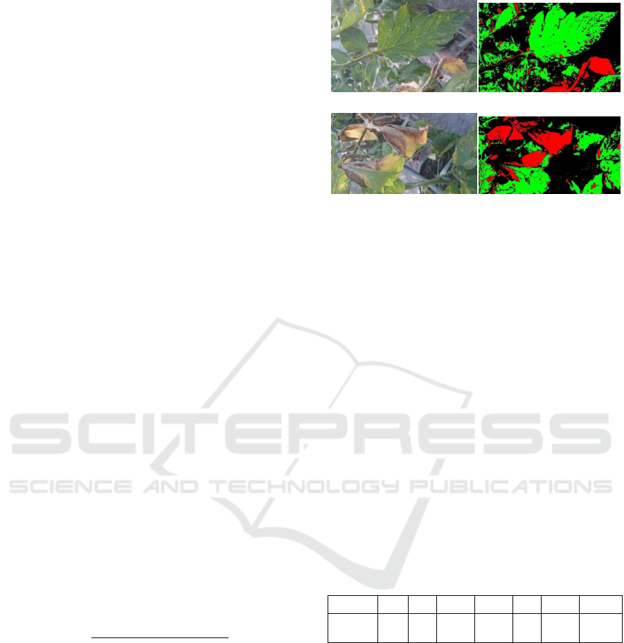
Figure 2: Examples of injured leaves from tomatoes, taken
in our experimental field, infected by P. infestans. The
images illustrate the images before and after the
classification process. Figure (2a) was accounted as
having a 15% of damage, or status 2, whereas Figure (2d)
was accounted for 32%, or status 4. It is important to
notice that the account was made considering the whole
group of leave captured by the camera, which was
considered to belong to the same plant.
Most of the pictures processed by the system
have a considerable number of background elements
that cause interference on the classification process.
Even after we reduced the noise by the mean-
filtering process, these background elements
remained, sometimes with the same color tonalities
of the healthy areas, and sometimes with the same
color tonalities of the sick areas of the plants. As our
goal is to use a drone to take the photos in the future
so we will try to deal automatically with those
problems in our next studies.
Table 1: Status for each range of damage percentage
(Correa et al., 2009).
Status
0
1
2
3
4
5
6
% of
damage
= 0
0-3
3-12
12-
22
22-
40
40-
76
>=77
5 THE DECISION SUPPORT
SYSTEM
According to the Integrated Pest Management
Program of California University (UCIPM, 2016),
there are several reputable prediction models of late
blight propagation in tomato and potato crops.
Among those, we have chosen the Hyre prediction
model (Hyre, 1954) that indicates that an initial
outbreak of late blight will occur between 7 to 14
days after 10 consecutive favorable days. A
ICEIS 2017 - 19th International Conference on Enterprise Information Systems
484
favorable day, in turn, occurs after five consecutive
days where the mean temperature stays between
7.0°C and 25.5°C (48°F and 78°F) and, at the same
time, after 10 days with a total precipitation equal to,
or higher than, 30 millimetres (1.2 inches).
5.1 The Forecasting Model
A forecasting model should perform multi-day
simulations and, for that reason, we needed to use up
to 40 days of meteorological prediction. To solve
that requirement, we have used historical data
obtained through the National Institute of
Meteorology (INMET, 2016). We have used that
data to calculate the mean of some meteorological
variables in specific periods of the year, chosen by
the system user during the simulation. We tested the
system with data from the city of Paty do Alferes,
because this is the main tomato producer region in
the State of Rio de Janeiro. Thus, we collected some
meteorological data from that region from
01/01/1999 until 01/01/2015, which includes
temperature, relative humidity, minimum
temperature, maximum temperature and
precipitation.
The system user can choose the size of the data
window that will be used in the historical average
calculation, and it can be 5, 10 or 15 years, for all
available variables. Finally, those historical averages
are used to estimate the meteorological variables,
required for Hyre's model, for each day of the period
of simulation, as exemplified in Table 2.
5.2 The Cellular Automata Model
We have used a cellular automata (CA) to model the
dynamics of late blight, defined in the two-
dimensional domain, with Moore's neighbourhood
and a probabilistic transition function based on
Hyre’s prediction model.
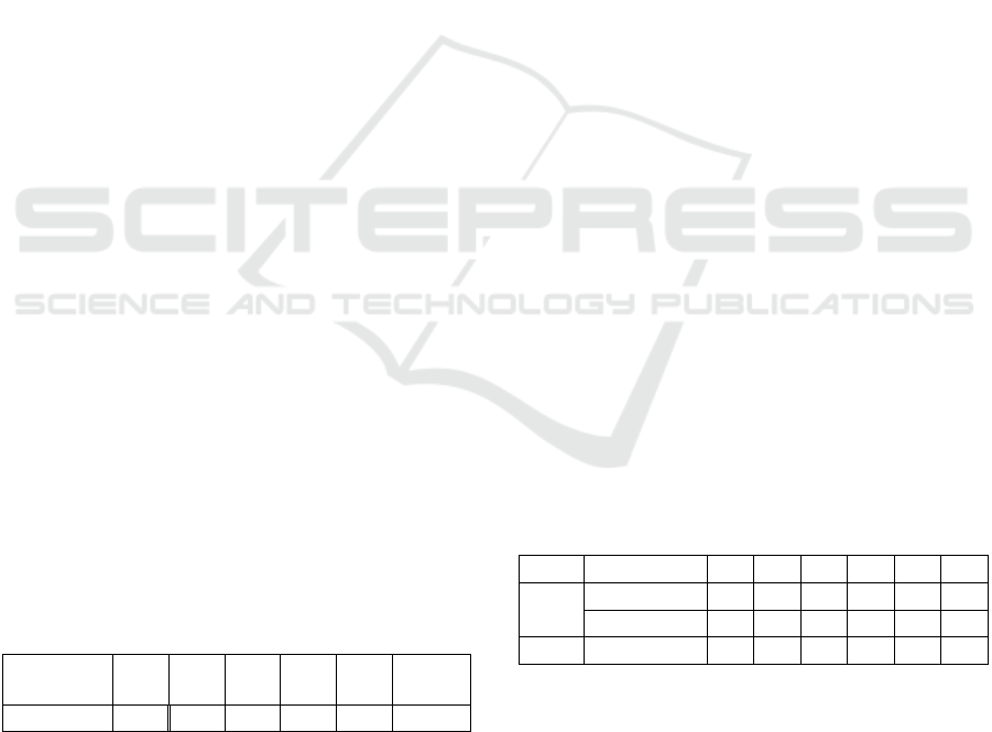
Table 2: Example of calculation of the expected
temperature for June 6
th
, 2016, using the historical average
temperatures and a 5-years window.
Simulation
Iteration
2010
2011
2012
2013
2014
Average
Result
06/06/16
17.42
11.24
21.64
18.48
16,88
17,13
The CA works over a matrix that represents a
cultivated area of tomatoes where the columns
correspond to lines of the cultivated area. Within
each column of the matrix the tomato plants are
arranged through the rows. Coherently, each cell in
the matrix represented a tomato plant that has a
health condition value, or status, associated with it.
The user defines the variable CA parameters, as
the size of the historical data window and the wind
direction. The parameter wind direction controls the
direction of the status changes. The status of any cell
would only change if it can be reached by an
infected cell in its neighbourhood and if the wind
direction allows this contact.
For each cell of the matrix, we calculated its
status in the next iteration by analysing the current
status of all its neighbors. The next status of a cell
c(i,j), where i is the line and j is the column, depends
on its current status, E(c(i,j)), and on the current
status of all its neighbors, in a neighborhood of size
8. An infected cell could have its status worsened
when there are infected cells in its neighbor, or
improved, when a technique C for combating the
disease is being used. Each neighbor can affect a cell
c(i,j) in a weighted way, according to the factors
indicated by Hyre’s model. The weighted influence
of each neighbor is calculated following the rules
shown in Table 3, which considered the number of
outbreaks Qo, the number of favorable days Qf, and
the current status E of cell c(I, j). Each cell in a
neighborhood would also change its value in the
next step, and the combination of all changes would
build the new status matrix.
We have tested two forms of combat and,
according to the literature (Rebouças et al., 2014), the
combat type 1, which uses Dimethimorph, could
decrease the status of a cell by 30% of the current
status. On the other hand, combat type 2, which uses
Metalaxyl-M+Mancozeb, could decrease the status
by 20%. Thus, when using a combat method, the CA
dynamics can be summarized by (2) and Table 3.
(2)
Table 3: Rules for calculation of weight P.
1
2
3
4
5
6
Qs> 1
Qd> = 10
0.1
0.8
1.4
1.6
1.8
2
10> Qd> = 7
0.1
0.5
1
1.1
1.2
1.4
Qs> 3
7> Qd> = 5
0.2
0.4
0.6
0.7
0.8
0.9
6 RESULTS AND DISCUSSION
The rules that control the simulation dynamics,
altering the cells status in order to represent the
spreading of late blight in the field are defined by a
set of parameters adjusted according to the Hyre’s
model.
A Neuro-automata Decision Support System for Phytosanitary Control of Late Blight
485
The simulation system is capable of mapping the
streets and lines of a farm, registering images and
georeferences of infected tomatoes. It can simulate
scenarios of contagion spreading in a determined
period from 10 up to 200 days. It is also possible to
stop the simulation at any time to choose a combat
method for the disease and then resume the
simulation. The system main functions are the
module for processing and classification of digital
tomato images described in previous sections, and
the simulator that generates scenarios of spreading of
contamination and alternatives to combat the disease.
In the module for processing and classification,
the images are classified within the status scale.
Thus, they are placed in a matrix based on their real
georeference information and the cell is painted with
a different color for each different status (Table 4).
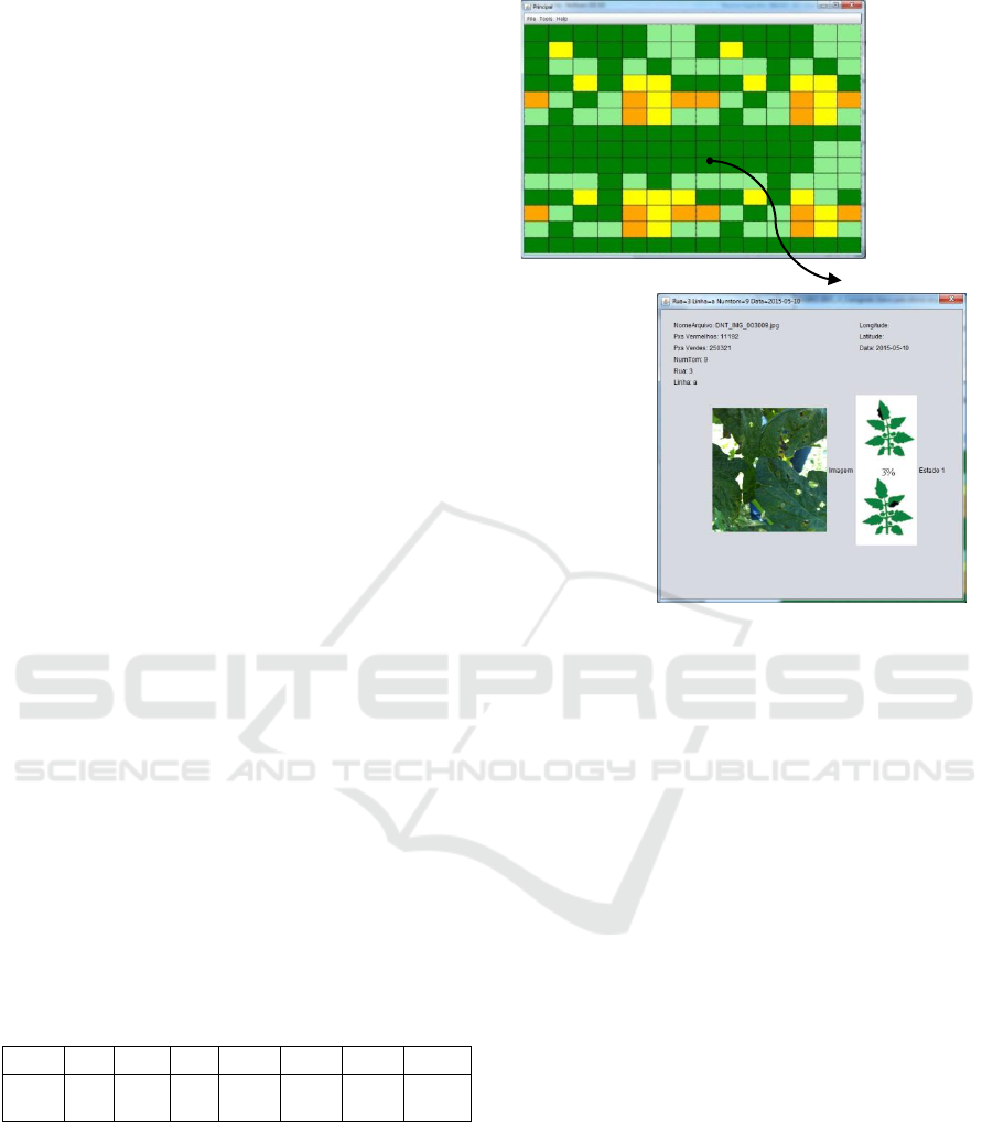
The resulting matrix thus conceptually represents
a map of the cultivated area being monitored by the
system (Figure 3a). In the map, it is possible to select
any cell and retrieve the corresponding sample
information, including the original leaf image, the
current health condition of the plant and the location
of the plant in the field (Figure 3b).
In the simulation module, it is possible to run
simulations of late blight spreading and visualize it
in the conceptual map of the cultivated area. It is
also possible to analyse strategies to combat the
disease. The simulation is interactive and simple,
and the user can pause, resume or restart the
simulation at any stage (Figure 4).
If a combat is tested during the simulation, a new
dynamic could occur, reducing the status of
tomatoes, depending on the contamination level of
the field as a whole, the climatic factors, and the
type of combat chosen. Figure 5 shows what
happens when combat type 2 is used on the 12
th
day
of simulation.
Table 4: correspondence of map cells for each possible
status.
Status
0
1
2
3
4
5
6
Cell
color
Dark
green
Green
Light
green
Yellow
Orange
Dark
Orange
Reddish
orange
Starting from the same situation of Figure 4a, it
is possible to see that the losses could be minimized
in the end of the 30
th
day of simulation.
(a)
(b)
Figure 3: (a) Conceptual map of a cultivated area of
tomatoes from a monitored farm. (b) Details from a
selected tomato on the map.
Our approach was to convert the original JPEG
images into codified red/green images, what proved
to be effective in highlighting the injuries of the
leaves (Bock et al., 2010). On the other hand, the
codification process was able to overcome problems
such as low resolution, focus, and image blur of the
digital images, with no need to use more
sophisticated digital image algorithms (e.g. contour
detection).
Since we have worked with images captured in
the field, in natural sunlight and taken by cell phones
cameras, it was expected that they would contain a
large amount of noise. As future work, we will
include more image filtering processes, aiming at
noise removal or attenuation.
ICEIS 2017 - 19th International Conference on Enterprise Information Systems
486

(a)
(b)
(c)
Figure 4: A non-combat simulation starting at 06/24/2016,
having wind direction from west to east and conducted
during 35 iterations on a matrix with 1200 elements,
where each cell represents one tomato plant. (a) At the
beginning, before the simulation starts, with cells
containing the original status of each plant, collected in
loco (cells marked with an ‘*’ represents one
photographed plant, while the others have their status all
settled to 0-healhy); (b) The map situation at iteration
number 12, which means that the map represents the farm
situation after 12 days from the initial day (c) The map
situation at the 35
th
day, when the simulation ends.
We are already working on a panel of statistics
that will show the performance of the simulation,
displaying the financial results obtained by chosen a
specific combat strategy, and comparing the costs of
using the pesticides against not using at all.
The alternative we presented can accelerate the
identification of the disease and help measuring the
extension of the infestation. Plus, it can help small
farmers to plan better the best time for spraying
fungicides, protecting the environment while
reducing the plantation costs.
We have modelled the dynamics of two chemical
fungicides to be available in this first version of our
simulator because they are the most common in
Brazil for tomato blight control. However, it is
relatively simple to model new chemical control
methods, and we are working on a tool that enables
the user to do so.
(a)
(b)
Figure 5; A combat type 2 simulation starting at
06/24/2016, having wind direction from west to east and
conducted during 35 iterations on a matrix with 1200
elements, where each cell represents one tomato plant. (a)
On the 12
th
day of simulation, the combat type 2 was
selected and the simulation was resumed; (b) The map
situation at iteration number 35, when the simulation ends.
A Neuro-automata Decision Support System for Phytosanitary Control of Late Blight
487

REFERENCES
Barbedo, J., 2013. Digital image processing techniques for
detecting, quantifying and classifying plant diseases.
In SpringerPlus, 2:660.
Bock, C., Poole, G., Parker, P., Gottwald, T., 2010. Plant
disease severity estimated visually, by digital
photography and image analysis, and by hyperspectral
imaging. In Critical Reviews in Plant Sciences, vol.
29, n. 1-3, pp.:59–107.
Bugiani, R. et al., 1995. Monitoring airborne
concentrations of sporangia of Phytophthora infestans
in relation to tomato late blight in Emilia Romagna,
Italy. In International Journal of Aerobiology, vol. 11,
, pp.:41-46, Elsevier Science.
Correa, F., Bueno, J., Carmo, M., 2009. Comparison of
three diagrammatic keys for the quantification of late
blight in tomato leaves. In Plant Pathology, vol. 58,
pp.:1128-1133.
Goufo, O., Mofor, T., Ngnokam, D., 2008. High Efficacy
of Extracts of Cameroon Plants Against Tomato Late
Blight Disease. In Agronomy for Sustainable
Development, vol. 8, INRA, EDP Sciences, pp.567-
573.
Hyre, R., 1954. Progress in forecasting late blight of
potato and tomato. In Plant Disease Reporter, Illinois,
vol. 38, n.4, pp.: 245-253.
IBGE, 2016. Sistema IBGE de Recuperação Automática –
SIDRA. [online] Available at: http://www.sidra.ibge.
gov.br/bda/agric/default.asp?z=t&o=11&i=P
[Accessed 18 Oct. 2016].
INMET, 2016. [online] Available at: http://
www.inmet.gov.br/portal/ [Accessed 5 Jun. 2016].
Mahlein, A., Oerke, E., Steiner, U., Dehne, H., 2012.
Recent advances in sensing plant diseases for
precision crop protection. In European Journal of
Plant Pathology, vol. 133, n.1, pp.:197-209.
MAPA, 2016. Estatísticas e Dados Básicos de Economia
Agrícola. [online] Available at: http://
www.agricultura.gov.br/arq_editor/Pasta%20de%20Se
tembro%20-%202016.pdf, [Accessed 10 Oct. 2016].
Mizubuti, E., Maziero, J., Maffia, L, Haddad, F., Lima,
M., 2002. CGTE Program: Simulation, Epidemiology
and Management of Late Blight. In Global Initiative
on Late Blight Conference, Hamburg, Germany.
Neves, E., Rodrigues, L., Dayoub, M., Dragone, D., 2003.
Bataticultura: dispêndios com defensivos agrícolas no
quinquênio 1997-2001. In Batata Show, vol. 6, pp. 22-
23.
Nixon, M., Aguado, A., 2008. Feature Extraction and
Image Processing, 2nd Ed, Elsevier Ltd.
Park, D., Zhang, Y., Kim, B., 2014. Improvement of
resistance to late blight in hybrid tomato. In Hort.
Environm. Biotechnol, vol. 55(2), Springer, pp.:120-
124.
Rebouças, T. et al., 2014. Potencialidade de Fungicida e
Agente Biológico no Controle da Requeima do
Tomateiro. In Horticultura Brasileira, vol.32(01).
Rembialkowska, E., 2007. Quality of plant products from
organic agriculture. In J. Sci. Food Agric., vol. 87,
pp.:2757–2762.
Sankaran, S., Mishraa, A., Ehsani, R., Davis, C., 2010. A
review of advanced techniques for detecting plant
diseases. In Computers and Electronics in Agriculture,
vol. 72, n.1, pp.:1-13.
Saxena, A., Sarma, B., Singh, H., 2014. Effect of
Azoxystrobin Based Fungicides in Management of
Chilli and Tomato Diseases. In Proced. National
Academy of Sciences, India:Springer.
Sevarac, Z., 2012. Neuroph - Java neural network
framework. [online] Available at: http://
neuroph.sourceforge.net/ [Accessed 10 Jan. 2012].
Tilman, D. et al., Agricultural sustainability and intensive
production practices, 2002. In Nature, Aug 8,
418(6898), pp.: 671-677.
UCIPM, 2016. [online] Available at:
http://www.ipm.ucdavis.edu/DISEASE/DATABASE/
potatolateblight.html [Accessed 9 Jun. 2016].
USDA, 2016. USABlight Project, [online] Available at:
https://usablight.org/node/29 [Accessed 4 Oct. 2016].
Vianna, G., Cruz, S., 2013a. Análise inteligente de
imagens digitais no monitoramento da requeima em
tomateiros. In Anais do IX Congresso Brasileiro de
Agroinformática. Cuiabá, Brazil.
Vianna, G.K., Cruz, S., 2013b. Redes neurais artificiais
aplicadas ao monitoramento da requeima em
tomateiros. In Anais do X Encontro Nacional de
Inteligência Artificial e Computacional (ENIAC),
Fortaleza, Brazil.
Vibhute, A., Bodhe, S.K., 2012. Applications of image
processing in agriculture: a survey. In International
Journal of Computer Applications, vol. 52, n.2,
pp.:34-40.
Zamberlan, F. et al., 2014. Produção e manejo agrícola:
impactos e desafios para sustentabilidade ambiental. In
Engenharia Sanitária Ambiental, Edição Especial, pp.
95-100.
Zhang, C. et al., 2013. Fine mapping of the Ph-3 gene
conferring resistance to late blight (Phytophthora
infestans) in tomato. In Theor. Appl. Genet., vol. 126,
Springer-Verlag, pp.:2643-2653.
Zhanga, N., Wangb, M., Wanga, N., 2002. Precision
agriculture-a worldwide overview. In Computers and
Electronics in Agriculture. vol. 36, issues 2-3,
pp.:113-132.
ICEIS 2017 - 19th International Conference on Enterprise Information Systems
488
