Shallow Networks for High-accuracy Road Object-detection

Khalid Ashraf, Bichen Wu,Forrest N. Iandola, Mattthew W. Moskewicz and Kurt Keutzer

Electrical Engineering and Computer Sciences Department, UC Berkeley, Berkeley, U.S.A.

Keywords:

Autonomous Driving, Vehicle Detection, Deep Learning.

Abstract:

The ability to automatically detect other vehicles on the road is vital to the safety of partially-autonomous

and fully-autonomous vehicles. Most of the high-accuracy techniques for this task are based on R-CNN or

one of its faster variants. In the research community, much emphasis has been applied to using 3D vision or

complex R-CNN variants to achieve higher accuracy. However, are there more straightforward modiﬁcations

that could deliver higher accuracy? Yes. We show that increasing input image resolution (i.e. upsampling)

offers up to 12 percentage-points higher accuracy compared to an off-the-shelf baseline. We also ﬁnd situations

where earlier/shallower layers of CNN provide higher accuracy than later/deeper layers. We further show that

shallow models and upsampled images yield competitive accuracy. Our ﬁndings contrast with the current

trend towards deeper and larger models to achieve high accuracy in domain speciﬁc detection tasks.

1 INTRODUCTION AND

MOTIVATION

Advanced driver assistance systems (ADAS) and in-

creasingly autonomous vehicles promise to make

transportation safe, efﬁcient and cost effective.

Driven by the goal of building a safe transportation

system, ADAS has emerged as a leading research

direction in recent years (Hillel et al., 2012; Hu-

val et al., 2015; Rajpurkar et al., 2015; Chen et al.,

2015a). Some speciﬁc ADAS related machine learn-

ing tasks include detection of road boundaries, lane

topologies, location of other cars, pedestrians, road

signs and obstacles. These detection capabilities form

the core of an ADAS technology stack. Other parts

of the technology stack include decision making and

control systems that take action in a certain road situ-

ation based on the input from the perception system.

Although this picture works in controlled environ-

ments, making this technology effective in changing

road situations, emergencies, changing weather etc.

remains a signiﬁcant challenge.

In recent times, deep learning has shown leading

accuracy in a number of machine learning challenges.

Speciﬁcally relevant to ADAS application is the dra-

matic increase in accuracy of image object classiﬁca-

tion (Krizhevsky et al., 2012; Szegedy et al., 2014;

Simonyan and Zisserman, 2014; He et al., 2015) and

localization (Sermanet et al., 2014; Zhu et al., 2015;

Girshick et al., 2014; Girshick, 2015; Ren et al., 2015)

in the last few years. A key advantage of DNN-based

approaches is that they do not require hand tuned fea-

tures for detecting every object but rather learn the

representation from the data itself. Deep learning

based perception systems promise to play a key role

in navigation and safety software stack for ADAS.

R-CNN and its faster variants have become the

state of the art in different object detection tasks. In

this work, we leverage this method to establish a num-

ber of observations related to car detection on the

challenging KITTI (Geiger et al., 2012) dataset. Our

main results can be summarized as:

• Bigger input images lead to higher accuracy.

Input image resolution increases the accuracy of

car detection using the faster R-CNN network.

• Shallow models can deliver high accuracy.

Convolutional features from shallow or earlier

layers of DNNs lead to higher accuracy than fea-

tures from the deeper layers. This holds true

for deep models like VGG16. Surprisingly, even

shallow models like AlexNet provide high accu-

racy on the detection task. Using shallow models

that require less memory allow us to use very high

input image resolutions. In terms of accuracy,

shallow models with high resolution are compet-

itive with deeper models with traditional resolu-

tion. This result is surprising given the trend of

searching for deeper models for achieving high

accuracy on object detection tasks.

The rest of the paper is organized as follows. In

Ashraf, K., Wu, B., Iandola, F., Moskewicz, M. and Keutzer, K.

Shallow Networks for High-accuracy Road Object-detection.

DOI: 10.5220/0006214900330040

In Proceedings of the 3rd International Conference on Vehicle Technology and Intelligent Transport Systems (VEHITS 2017), pages 33-40

ISBN: 978-989-758-242-4

Section 2 we review related work, and we provide

technical background information in Section 3. We

describe our initial experimental setup in Section 4.

We get to the crux of our results about large image

resolution in Section 5 and shallow models in Sec-

tion 6. We do additional exploration of R-CNN based

conﬁgurations in Section 7 We summarize our ﬁnd-

ings in the context of the related work in Section 8,

and we conclude in Section 9.

2 RELATED WORK

2.1 Deep Networks for Object Detection

Deformable parts models (DPM) were the state of the

art for image object detection (Felzenszwalb et al.,

2010) before the emergence of deep convolutional

neural nets. The R-CNN method uses selective search

for object region proposal (Girshick et al., 2014). The

proposed regions in an image are warped to a ﬁxed

size and fed into a classiﬁcation network called R-

CNN. Fast R-CNN was introduced to reuse the shared

convolution features for the region proposals (Gir-

shick, 2015). In Fast R-CNN (Girshick, 2015), the in-

ference speed is still dominated by the region proposal

in the selective search method. Faster R-CNN (Ren

et al., 2015) proposes object bounding boxes directly

from the convolutional features. Inspired by the SPP-

Net (He et al., 2014) method, Faster R-CNN uses a

region proposal network (RPN) to regress proposal

boxes to ground truth boxes. The regions proposed

by the RPN network is fed into the R-CNN network

for classiﬁcation. The network is trained end to end.

Other than the RPN based method, there are several

methods proposed for object bounding box predic-

tion. For example, the OverFeat (Sermanet et al.,

2014) method predicts a single box for localization

whereas the Multibox (Erhan et al., 2014; Szegedy

et al., 2015) method predicts multiple boxes in a class-

agnostic way. The SPP method (He et al., 2014) uses

shared convolutional feature maps for fast object de-

tection.

2.2 Detection on the KITTI Dataset

2.2.1 Detection using 2D Data

Deep neural networks are the backbone of most high-

accuracy approaches to identifying objects such as

The Faster R-CNN codebase also offers piecewise

training of RPN and classiﬁer branches of the network, but

we found this cumbersome, and we use end-to-end training

in all of our Faster R-CNN experiments.

cars in KITTI and similar datasets. Many such meth-

ods have been proposed; we focus this section on

the high-accuracy and peer-reviewed results. A high-

accuracy method for identifying objects in KITTI

dataset is scale dependent pooling (SDP) combined

with cascaded region classiﬁers (CRC) (Yang et al.,

2016). The crux of SDP+CRC lies in selecting a high-

resolution CNN layer (e.g. conv3 3 in VGG16 (Si-

monyan and Zisserman, 2014)) or a heavily down-

sampled CNN layer (e.g. conv5 3), depending on the

resolution of each region proposal. By combining fea-

tures from multiple convolution layers, they were able

to achieve very high accuracy on KITTI’s object de-

tection task. Our method introduced in this paper is

even simpler in that we use only a single layer for

feature extraction.

Another approach is Monocular 3D (Mono3D)

which actually uses 2D images, but it aims to identify

the pose of objects, with the goal of detecting objects

as 3D bounding boxes. Like SDP+CRC, Mono3D is

built around a version of R-CNN. There are also a

number of anonymous and/or sparsely-explained sub-

missions to the KITTI website’s leaderboard that are

reportedly built on top of R-CNN.

2.2.2 Detection using 3D Data

The KITTI dataset provides 3D information in the

form of stereo images and LIDAR point clouds. Re-

cent results such as 3DVP (Xiang et al., 2015) and

3DOP (Chen et al., 2015b) leverage both 2D and 3D

data to achieve higher accuracy relative to comparable

2D baselines.

To build supervised 2D datasets such as Ima-

geNet (Deng et al., 2009) and PASCAL (Everingham

et al., 2010), a widely-used approach is to have me-

chanical turk workers annotate user-generated images

and videos from websites such as Flickr or YouTube.

However, to our knowledge, there is no 3D equivalent

of Flickr or YouTube that receives petabytes per week

of user-uploaded 3D imagery. As a result, the over-

head in building a 3D dataset currently requires not

only data annotation, but also data collection. The

cost of data collection includes hours of human la-

bor, and it can also require expensive sensors. The

KITTI dataset was released several years ago. How-

ever, the Velodyne HDL-64E LIDAR scanner used

by the KITTI team still costs 80,000 USD

, which

is more than twice the price of the average new car

in the United States. With all of this in mind, we

think widespread research on 3D object detection will

be slow to emerge until (1) there is an internet hub

that attracts large quantities of user-generated 3D im-

http://articles.sae.org/13899

VEHITS 2017 - 3rd International Conference on Vehicle Technology and Intelligent Transport Systems

agery, and (2) the equivalent of today’s high-end LI-

DAR sensors become available for tens of US dollars.

With this in mind, we focus our efforts on 2D im-

agery, where anyone with modest resources can col-

lect a custom training set and apply our object detec-

tion approach.

3 PRELIMINARIES

3.1 Relationship of Conv and Pooling

Strides to Activation Grid

Dimensions

The feature dimension of the output of a spatial con-

volution operation depends on the dimension of its

input and the strides used (ignoring the boundary ef-

fects). In convolutional neural nets, strides are used

to continually reduce the feature dimensions in the

convolution layers. Additionally pooling layers are

used to reduce dimension by averaging or taking max-

imum value within a neighborhood. Thus the spatial

dimension of the output of the convolution decreases

as we go to deeper layers. For example, in VGG16,

for a standard input image size 224x224, the features

calculated by the ﬁrst convolution layer is 224x224

which reduce to 14x14 at the output of conv5 3. This

dimension is further reduced by the pool5 layer to

7x7. Similarly for AlexNet, the convolution feature

dimension reduces from 55x55 in conv1 to 6x6 in

pool5.

In some CNN architectures such as

AlexNet (Krizhevsky et al., 2012) and VGG16 (Si-

monyan and Zisserman, 2014), the ﬁrst fully-

connected layer expects a speciﬁc height and width

for its input data (e.g. 6x6 for AlexNet). Increasing

the height and width of the input image results in a

higher-resolution input to the ﬁrst FC layer. At the

CNN architecture level, an easy way around this is

to design a CNN architecture that has global average

pooling prior to the ﬁrst FC layer – this approach

was popularized in the Network-in-Network (NiN)

architecture (Lin et al., 2013), and it is now used

in other architectures such as SqueezeNet (Iandola

et al., 2016) and ResNet architectures (He et al.,

2015). However, when using AlexNet or VGG19, the

R-CNN authors developed a technique called ROI

Pooling that allows any size input image to be used in

concert with AlexNet/VGG FC layers. ROI pooling

is quite simple: no matter what the input image size

is, ROI Pooling uses max-pooling to reshape the ﬁrst

FC layer’s input to the size that it expects.

3.2 Region Proposal Network in Faster

R-CNN

We brieﬂy review how the region proposal network

(RPN) in Faster R-CNN generate proposals (Ren

et al., 2015) that will be useful later. RPN starts with

convolution layers, which computes a high dimen-

sional, low resolution feature map for the input image.

Next, a small network slides through each spatial po-

sition in the feature map and generates rectangular re-

gion proposals centered around the position. Instead

of computing the proposal’s absolute coordinates, the

RPN actually computes coordinates relative to a set of

k pre-selected reference boxes, or anchors. The trans-

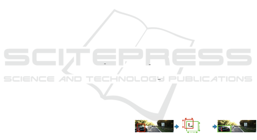
formation from an anchor to a proposal is illustrated

in Fig. 1.

Intuitively, we want the anchors to be spatially

close to the ground truth bounding boxes. In an ex-

treme case, if an anchor box is too far away from the

ground truth bounding box, learning to transform the

anchor to the ground truth will be hopeless. Since

anchors are centered at each spatial position on the

feature map, and each position on the feature map

corresponds to a patch of pixels on the original im-

age, the resolution of the feature map affects the dis-

tance from a ground truth bounding box to its near-

est anchor. In VGG16, for example, each position in

conv5 3 layer spatially corresponds to a 16 ×16 patch

on the original image, so in the worst case, the nearest

anchor to the center of a ground truth bounding box

is 16 ×

√

2/2 ≈ 11.31. As we will see later in this

paper, reducing this distance, or relatively, increasing

the “anchor density” will signiﬁcantly increase the lo-

calization accuracy, thus improve the detection accu-

racy.

exp(w)

exp(h)



Anchor box

Box transformation

Proposal box

Figure 1: Transformation from an anchor box (left) to a

proposal (right). 4 relative coordinates are regressed by the

RPN network to adjust the center position and the shape of

the bounding box.

4 EXPERIMENTAL SETUP

4.1 Networks and Training

Conﬁguration

We train faster R-CNN networks built on the

VGG16 (Simonyan and Zisserman, 2014) and

AlexNet (Krizhevsky et al., 2012), pretrained on

Shallow Networks for High-accuracy Road Object-detection

the ImageNet-1k (Deng et al., 2009) classiﬁcation

dataset. VGG16 has sixteen convolution layers (Si-

monyan and Zisserman, 2014) and AlexNet has only

ﬁve convolutional layers (Krizhevsky et al., 2012).

Rather than using the convolution features of the last

pooled layer (as is done in the original faster R-CNN

paper), we use features from convolutional layers that

are the bottom layers of the previous pooling layer.

For VGG16 it is conv4 3. We resize the roipooling

window size accordingly. For VGG16 the window

size changes from 7x7 to 13x13. We also reduce the

feature stride by a factor of two for avoiding one pool-

ing stage. For VGG16 and AlexNet, fully connected

layers are used as the R-CNN branch. The weights

in these layers are initialized with random gaussian

noise. As the standard procedure introduced in faster

R-CNN, we randomly sample 128 positive and 128

negative roi proposals per batch to train the R-CNN

layer. For all the experiments, we use initial learning

rate of 0.0005, step size 50000 and momentum 0.9.

A total of 70K iterations are run during R-CNN train-

ing starting from imagenet pre-trained weights for the

convolution layers.

4.2 Dataset

We use the KITTI object detection dataset. KITTI

object has three categories that is car, pedestrian, bi-

cyclists. The dataset is annotated in three categories

based on the occlusion and truncation of the objects.

The hard category is heavily occluded and truncated

whereas the easy category is relatively clearly visi-

ble. There are about 8000 images for both training

and testing. The moderate regime is used to rank the

competing methods in the benchmark. Our split of the

KITTI train and validation sets (each containing half

of the images) is the same as (Chen et al., 2015b).

The evaluation criteria is the same that is prescribed in

the KITTI development kit. In KITTI’s evaluation cri-

teria, proposal boxes having overlap with the ground

truth or IoU greater than 70% are counted as true de-

tection for cars.

The Faster R-CNN algorithm has been shown

to deliver high accuracy on the PASCAL (Evering-

ham et al., 2010) dataset. Adapting that pipeline

from PASCAL to KITTI poses a few natural chal-

lenges. First, the image sizes in the KITTI dataset

is 1242x375 pixels whereas the image sizes in PAS-

CAL dataset is 500 pixels in the longest dimension

(many PASCAL images are 500x333 or 333x500).

More importantly, the KITTI dataset contains heavily

occluded and truncated objects. These objects come

in multiple scales. The presence of objects at mul-

tiple scales make it difﬁcult to attain high accuracy

specially for small objects.

5 INPUT IMAGE RESOLUTION

We performed extensive design space search of Faster

R-CNN conﬁgurations on the KITTI dataset. Our

starting point is the VGG16 network that has achieved

high accuracy in both image classiﬁcation (Simonyan

and Zisserman, 2014) and localization (Ren et al.,

2015). We performed an input image scaling exper-

iment to ﬁnd its impact on the accuracy. In these ex-

periments, the shorter side of the KITTI images were

ﬁxed at 1295 pixels. In the Faster R-CNN codebase,

the default off-the-shelf conﬁguration resizes all im-

ages to 1000 pixels in the long dimension.

KITTI images have a native resolution of

1295x375, so the default Faster R-CNN behavior is to

resize KITTI images to 1000x302. But, is this resiz-

ing scheme ideal for obtaining high accuracy? To ﬁnd

out, we doubled the input image height and width to

2000x604. This has the effect of doubling the height

and width of the activations (outputs) from all convo-

lutional layers. For example, the conv5 3 activations

– which serves as input to both the region proposal

network (RPN) and the classiﬁcation network – dou-

ble in height and width. With the image upsampled

to 2000x604, we see in Table 1 that the KITTI car-

detection accuracy increases for easy, medium, and

hard by 7.1, 15.5, and 12.6 percentage points, respec-

tively. In a world where half of a percentage point is

considered signiﬁcant, we can say with certainty that

the input resolution has a major impact on accuracy.

Can further upsampling of the image lead to

further improvements in accuracy? We attempted

to perform experiments with upsampling beyond

2000x604, but the volume of activation planes ex-

ceeded the 12GB of available memory on an NVIDIA

Titan X GPU. In the next section, we consider shal-

lower networks with fewer layers of activation planes,

which enables us to move to even higher input resolu-

tions.

Table 1: KITTI car detection accuracy using different in-

put image sizes to VGG16. In these experiments, we use

conv5 3 features from VGG16.

Input resolution Easy Medium High

1000x302 80.3 63.0 52.3

2000x604 87.4 78.5 64.9

VEHITS 2017 - 3rd International Conference on Vehicle Technology and Intelligent Transport Systems

6 SHALLOW CONVOLUTIONAL

MODELS

So far, we have upsampled the input image until we

ran out of on-chip GPU memory when training R-

CNN models with a VGG16-based feature representa-

tion. Based on what we have seen so far, it seems that

further upsampling may lead to further gains in ac-

curacy. We need to ﬁnd a conﬁguration that requires

less memory for a given image size, and then we will

exploit this extra memory to further upsample the im-

age. One idea would be to decrease the batch size to

save memory, but we are already using a batch size of

1, and it’s not clear how to reduce the batch size below

1. Could we reduce the memory footprint by reducing

the number of layers in the CNN? Much of the recent

literature shows that fewer layers in a CNN leads to

lower accuracy (all else held equal). But, our goal

is to conﬁgure a CNN with fewer layers (and mod-

erately lower accuracy) and then increase the input

image resolution (leading to much higher accuracy).

To evaluate this idea, we conﬁgure R-CNN to use

2000x604 images (2x height and 2x width compared

to our original starting point), using conv4 3 instead

of conv5 3 features. In VGG16’s scheme for naming

layers, conv4 3 is the 10th layer, and conv5 3 is the

13th layer in the CNN. We expected that the accuracy

of R-CNN with conv4 3 would be slightly lower than

R-CNN with conv5 3, but as we show in Table 2 that

the accuracy is higher with conv4 3 by 5.5, 9.4, and

12.4 percentage-points for easy, medium, and hard

detections. Cumulatively, the improvement in accu-

racy from conv5 3 with 1000x302 images to conv4 3

with 2000x604 images is a whopping 12.6, 24.9, and

25.0 percentage-points for easy, medium, and hard,

respectively.

How does further reducing the CNN’s depth af-

fect accuracy? We initially considered using the ear-

lier layers of VGG16 as input to the Region Proposal

Network. But, earlier layers in VGG16 have been

downsampled less, so their activations have a larger

height and width. We found that the off-the-shelf

implementation of RPN comes to dominate the end-

to-end computation time with very large height and

width input grids. Besides depth, one of the differ-

ences between VGG16 and AlexNet is that AlexNet

downsamples more aggressively in the early layers –

for example AlexNet has stride=4 in the conv1 layer

(4x downsampling), while the conv1 layer of VGG16

has stride=1 (no downsampling). So, to evaluate this

question of how using shallower (<10 conv layers)

network impacts accuracy, we use AlexNet instead

of VGG16. We use conv5 (5th layer) activations as

input to the R-CNN region-proposal and classiﬁca-

tion branches, and we report the results in Table 2.

With resolution of 2000x604 for both AlexNet-conv5

and VGG16-conv4 3, the VGG16-based conﬁgura-

tion delivers signiﬁcantly higher accuracy on easy,

medium, and hard detections in Table 2. We have

additional memory available when running AlexNet

with 2000x604 input images, so we now try upsam-

pling the AlexNet input images to 5000x1510. In this

conﬁguration, on the easy detections, AlexNet with

5000x1510 input is within 0.5 of a percentage-point

of our best VGG16-based result so far. On medium

and hard categories, VGG16 conv4 3 with an input

resolution of 2000x604 delivers higher accuracy than

AlexNet with 2000x604 or 5000x1510 input images.

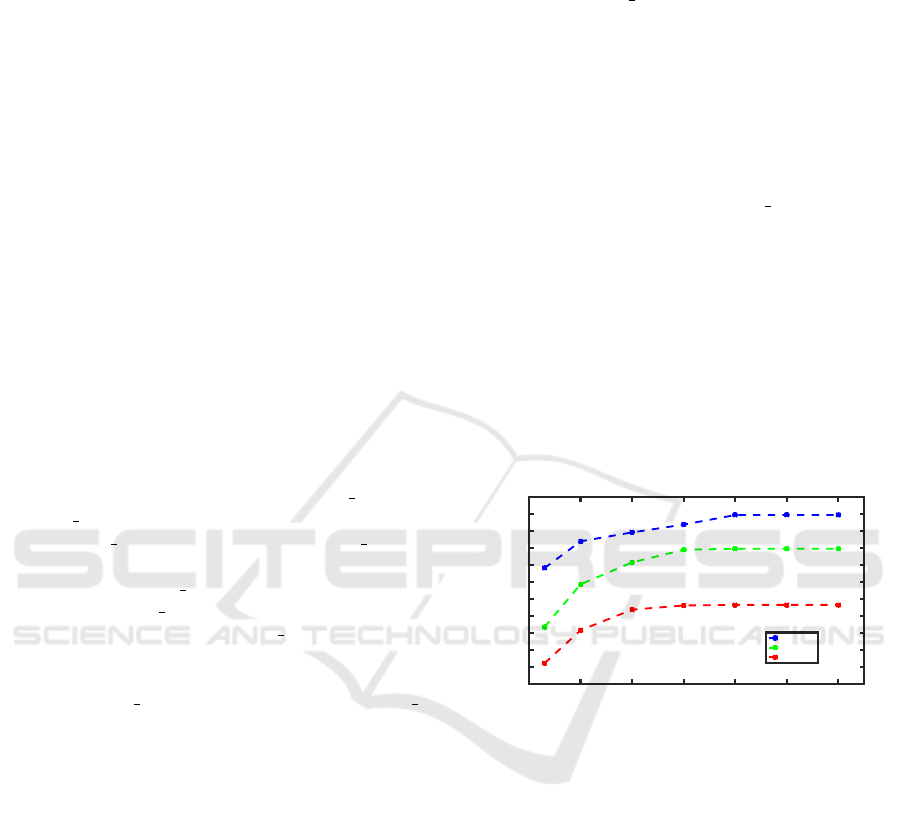
We also conduct a sweep of input image sizes ap-

plied to an AlexNet-based R-CNN model that uses

conv5 features. We show the results of this sweep

in Figure 2. We observe that KITTI car detection

accuracy steadily climbs from a baseline resolution

of 1000x302 to a plateau at resolution 5000x1510.

Beyond this resolution, we have not observed fur-

ther accuracy improvements at larger sizes such as

6000x1811 or 7000x2133.

1000 2000 3000 4000 5000 6000 7000

Image width (pixels)

100

Average precision (%)

easy

medium

hard

Figure 2: Evaluation of how input resolution affects accu-

racy on KITTI car detection. In this conﬁguration, we use

AlexNet conv5 as input features to the R-CNN branches.

7 FURTHER IMPROVEMENTS

7.1 Context Windows

Chen et al. (Chen et al., 2015b) proposed context win-

dows as a way to include information from adjacent

pixels of a proposed bounding box. A context window

is a bounding box that is scaled up from the original

bounding box proposal of the RPN network. In the

experiments with context window, in addition to the

original R-CNN branch, an extra R-CNN branch

is added that trains on the features extracted from

context window. The original R-CNN features and

the context R-CNN features are concatenated before

classiﬁcation. We add a context branch in addition to

Shallow Networks for High-accuracy Road Object-detection

Table 2: Impact of CNN depth on accuracy. Conventional wisdom would suggest that deeper representations would produce

higher accuracy, but we ﬁnd otherwise. AP numbers are for car detection on the KITTI dataset.

CNN Architecture Conv layer name (depth) Input image resolution Easy Medium Hard

VGG16 conv5 3 (13) 2000x604 87.4 78.5 64.9

VGG16 conv4 3 (10) 2000x604 92.9 87.9 77.3

AlexNet conv5 (5) 2000x604 86.7 71.6 56.1

AlexNet conv5 (5) 5000x1510 92.4 82.5 68.2

Table 3: Impact of anchor box shape on accuracy. These results use AlexNet conv5 features.

DNN architecture Input resolution Anchor shape selection scheme AP

Easy Moderate Hard

AlexNet 1242x375 Default shape 70.37 54.44 46.33

AlexNet 1242x375 K-Means 76.12 59.29 47.38

AlexNet 2500x755 Default shape 84.12 72.14 58.29

AlexNet 2500x755 K-Means 83.27 71.43 62.42

AlexNet 5000x1510 Default shape 91.33 84.52 69.90

AlexNet 5000x1510 K-Means 91.44 85.98 70.04

Table 4: Summary of results on KITTI (Geiger et al., 2012) car detection. All of our results are based on Faster R-CNN. To

our knowledge, all of the related work discussed in this table also uses a version of R-CNN.

Source CNN

Architecture

Feature layer

(Depth)

Input

resolution

Context

window

Easy Medium Hard

SDP+CRC (Yang et al.,

2016)

VGG16 conv3 3, 4 3, 5 3

(7,10,13)

multiple no 90.3 83.5 71.1

Mono3D (Chen et al.,

2016)

VGG16 conv5 3 (13) not reported yes 92.3 88.7 79.0

ours VGG16 conv5 3 (13) 1000X302 no 80.25 62.96 52.3

ours VGG16 conv5 3 (13) 2000X604 no 87.35 78.49 64.93

ours VGG16 conv4 3 (10) 2000X604 no 92.9 87.9 77.3

ours VGG16 conv4 3 (10) 5000x1510 no out of memory

ours AlexNet conv5 (5) 1000X302 no 67.5 49.44 38.9

ours AlexNet conv5 (5) 2000X604 no 86.7 71.6 58.1

ours AlexNet conv5 (5) 5000x1510 no 92.4 82.5 68.2

ours AlexNet conv5 (5) 1000X302 yes 71.58 51.13 40.9

ours AlexNet conv5 (5) 2000X604 yes 86.98 74.32 60.83

ours AlexNet conv5 (5) 5000x1510 yes 94.7 84.8 68.3

the usual R-CNN branch with a spatial bounding box

scaling of 1.5. When applying the context window to

an AlexNet-based R-CNN conﬁguration, we ﬁnd that

the accuracy of all the categories improve as shown

in Table 4. The improvement is signiﬁcant in small

image sizes and provides diminishing returns as we

scale up the input image size.

7.2 Optimal Anchor-box Shape

In (Ren et al., 2015), default anchor shapes are arbi-

trarily chosen by reshaping a 16 ×16 square box by

3 scales and 3 aspect ratios. But is there a better way

to choose anchor shapes for input images and target

objects? Intuitively, we want the anchors to have sim-

ilar shapes with the ground truth bounding boxes. The

shape of a bounding box can be characterized by its

width w and its height h. The width and height dis-

tribution of the car object in the KITTI training data

set is plotted in Fig. 3(a). The problem of choosing

the ”most similar” k anchor shapes can be formulated

as the following: given a set of ground truth bound-

ing box shape observations {(w

)}, ﬁnd k anchors

such that the sum of the distance (in the shape space

of (width,height)) between each ground truth box to

its nearest anchor is minimized. This problem can be

effectively solved by K-means. The optimal anchor

shapes are plotted in Fig. 3(b). These anchors are op-

VEHITS 2017 - 3rd International Conference on Vehicle Technology and Intelligent Transport Systems

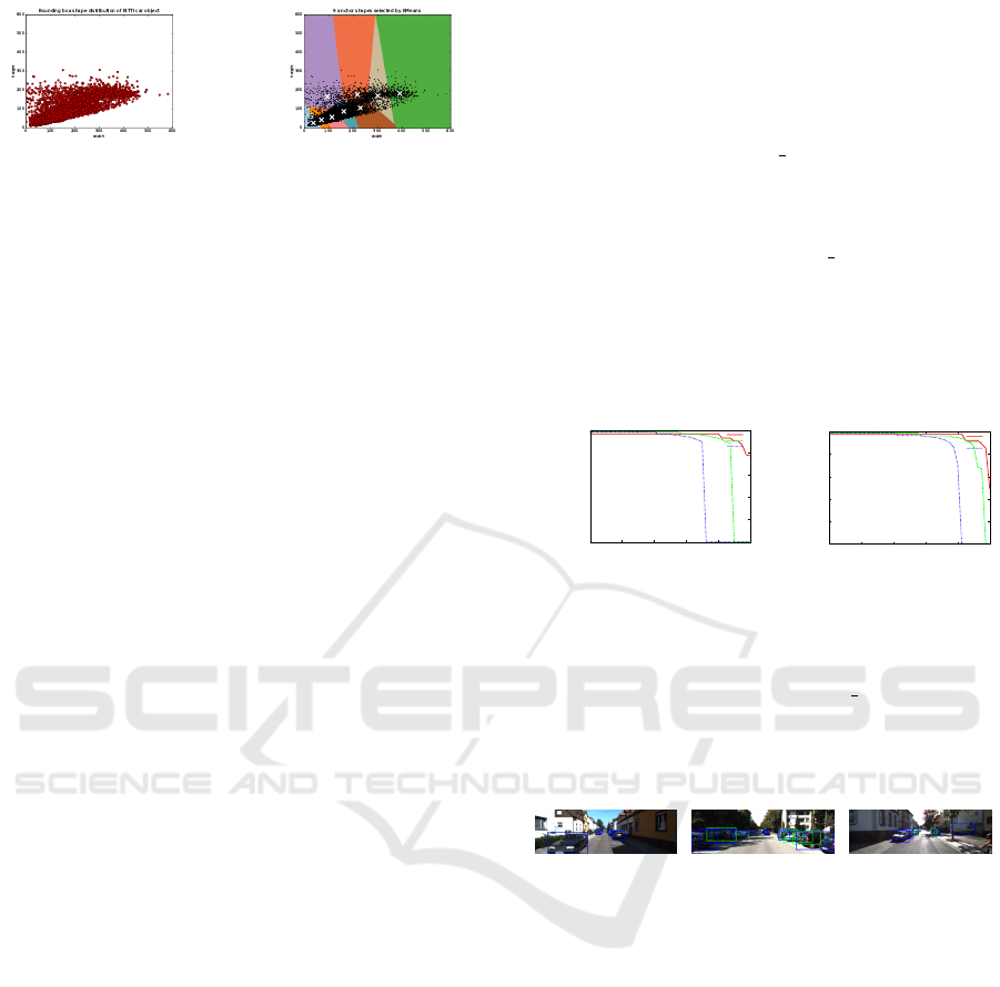
(a) Distribution of

bounding box shapes

of cars in the KITTI

dataset

(b) 9 Anchor box

shapes (white crosses)

selected by K-Means

Figure 3: Bounding box shape distribution of the car ob-

ject in the KITTI dataset is plotted on the left. 9 anchor

shapes computed by K-Means are plotted in the right ﬁgure

as white crosses.

timized speciﬁcally for the car category, but the idea

of optimizing anchors by considering ground truth

bounding box statistics can be generalized to multi-

category object detection as well.

We tested the AlexNet-based Faster R-CNN’s de-

tection accuracy with different anchor box selection

schemes, and the result is shown in Table 3. We ﬁx

the number of anchors to be 9. From the bounding

box shapes of cars in the training data set, we used K-

Means to select 9 optimal anchor boxes. As compari-

son, we used a set of default anchors with 3 scales and

3 aspect ratios as in (Ren et al., 2015). When image

width is 1242, using the K-Means selected anchors

improves AP signiﬁcantly comparing with the default

anchors. When the image width is 2500, we could

see that AP with default shapes are slightly better for

easy and moderate category, but using K-Means se-

lected anchors still improves AP for the hard category

by 4 percentage points. As we further scale the im-

age width to 5000, the performance gain saturates, we

still observe some improvement by using K-Means

selected anchors. We have not yet combined context

windows with our anchor box improvements, but it

is possible that this combination will yield a further

improvement in accuracy.

8 DISCUSSION

We show the precision-recall curve for our KITTI

car detection in Fig. 4(a). We used AlexNet-conv5

with a context window and input image resolution of

5000x1510, as in the ﬁnal row of Table 4. We ob-

serve that the precision of the easy category is very

high even at very high recall. However, the precision

in the hard category suffers at high recall. Improv-

ing the precision of results on the hard category with

our method will be a target of future work. We show

a few examples of success and failure modes in the

hard category in Fig 5. In Fig 5(a), the model suc-

cessfully predict a highly occluded car while in Fig

5(b) the predicted bounding box encompass two cars

that are adjacent to each other. In Fig 5(c), the pre-

dicted bounding box enclose a visible car but com-

pletely misses the car that is truncated. The precision-

recall curve using the conv4 3 features of VGG16 is

shown in Fig.4(b). The precision at high recall for the

hard category improves signiﬁcantly. The inference

time using AlexNet conv5 layer with input image size

of 5000x1510 and VGG16 conv4 3 layer with input

image size of 2000x604 is 0.34s and 0.6s respectively.

Inference times for other published high accuracy

methods on the KITTI dataset are 3s for 3DOP (Chen

et al., 2015b) and 0.4s for SDP+CRC (Yang et al.,

2016).

0.2

0.4

0.6

0.8

0 0.2 0.4 0.6 0.8 1

Precision

Recall

Car

Easy

Moderate

Hard

(a) Precision-recall curve

for the AlexNet network

with context window. The

input image size is 5000.

The conv5 features are

used in this experiment.

0.2

0.4

0.6

0.8

0 0.2 0.4 0.6 0.8 1

Precision

Recall

Car

Easy

Moderate

Hard

(b) Precision-recall

curve for the VGG16

network without con-

text window. The input

image size is 2000. The

conv4 3 features are

used in this experiment.

Figure 4: Precision vs. recall curve for KITTI’s car detec-

tion system.

(a) Success. (b) Predicting

one box for two

adjacent cars.

Figure 5: Examples of success(a) and failure modes(b,c) in

the hard category using AlexNet conv5 with a context win-

dow and input resolution of 5000x1510 pixels. The green

boxes show the ground truth label of heavily truncated car.

In (a), the model successfully predict a highly occluded car.

In (b), the predicted bounding box encompass two cars that

are adjacent to each other. In (c), the predicted bounding

box enclose a visible car but completely misses the car that

is truncated.

9 CONCLUSIONS

In summary, we have shown that shallow networks

perform well in achieving high accuracy on detect-

ing cars in the road. We have shown that input image

resolution has a large impact on the accuracy of car

detection using the faster R-CNN network. For very

deep models, shallow layers can (surprisingly) pro-

Shallow Networks for High-accuracy Road Object-detection

vide higher accuracy than the later convolutional lay-

ers deep in the network. Shallow models like AlexNet

can achieve high accuracy when the input image is

upsampled. In addition, we have used an anchor box

selection method and context window to further en-

hance car detection accuracy. We believe that our

ﬁndings will inspire the research community to eval-

uate shallow models for achieving high accuracy on

object detection tasks.

ACKNOWLEDGMENTS

Khalid Ashraf was supported by the National Sci-

ence Foundation under Award number 125127. We

thank Kostadin Ilov for many help with computational

hardware. Thanks to Ross Girshick for comments on

some initial results. Thanks to Fan Yang and Kaustav

Kundu for clariﬁcation on their results.

REFERENCES

Chen, C., Seff, A., Kornhauser, A., and Xiao, J. (2015a).

Deepdriving: Learning affordance for direct percep-

tion in autonomous driving. In CVPR.

Chen, X., Kundu, K., Zhang, Z., Ma, H., Fidler, S., and

Urtasun, R. (2016). Monocular 3d object detection

for autonomous driving. In CVPR.

Chen, X., Kundu, K., Zhu, Y., Berneshawi, A., Ma, H., Fi-

dler, S., and Urtasun, R. (2015b). 3d object proposals

for accurate object class detection. NIPS.

Deng, J., Dong, W., Socher, R., Li, L.-J., Li, K., and Fei-

Fei, L. (2009). ImageNet: A large-scale hierarchical

image database. In CVPR.

Erhan, D., Szegedy, C., Toshev, A., and Anguelov, D.

(2014). Scalable object detection using deep neural

networks. In CVPR.

Everingham, M., Gool, L. V., Williams, C. K. I., Winn,

J., and Zisserman, A. (2010). The pascal visual ob-

ject classes (voc) challenge. International Journal of

Computer Vision (IJCV).

Felzenszwalb, P., Girshick, R., McAllester, D., and Ra-

manan, D. (2010). Object Detection with Discrimi-

natively Trained Part Based Models. PAMI.

Geiger, A., Lenz, P., and Urtasun, R. (2012). Are we ready

for autonomous driving? the kitti vision benchmark

suite. In CVPR.

Girshick, R. (2015). Fast r-cnn. In ICCV.

Girshick, R. B., Donahue, J., Darrell, T., and Malik, J.

(2014). Rich feature hierarchies for accurate object

detection and semantic segmentation. In CVPR.

He, K., Zhang, X., Ren, S., and Sun, J. (2014). Spatial

pyramid pooling in deep convolutional networks for

visual recognition. arXiv:1406.4729.

He, K., Zhang, X., Ren, S., and Sun, J. (2015). Deep resid-

ual learning for image recognition. arXiv:1512.03385.

Hillel, A. B., Lerner, R., Levi, D., and Raz, G. (2012). Re-

cent progress in road and lane detection: a survey. Ma-

chine Vision and Applications.

Huval, B., Wang, T., Tandon, S., Kiske, J., Song, W.,

Pazhayampallil, J., Andriluka, M., Rajpurkar, P.,

Migimatsu, T., Cheng-Yue, R., Mujica, F., Coates,

A., and Ng, A. Y. (2015). An empirical evaluation

of deep learning on highway driving. arXiv preprint

arXiv:1504.01716v3.

Iandola, F. N., Moskewicz, M. W., Ashraf, K., Han, S.,

Dally, W. J., and Keutzer, K. (2016). Squeezenet:

Alexnet-level accuracy with 50x fewer parameters and

<1mb model size. arXiv:1602.07360.

Krizhevsky, A., Sutskever, I., and Hinton, G. E. (2012). Im-

ageNet Classiﬁcation with Deep Convolutional Neu-

ral Networks. In NIPS.

Lin, M., Chen, Q., and Yan, S. (2013). Network in network.

arXiv:1312.4400.

Rajpurkar, P., Migimatsu, T., Kiske, J., Cheng-Yue, R., Tan-

don, S., Wang, T., and Ng, A. (2015). Driverseat:

Crowdstrapping learning tasks for autonomous driv-

ing. arXiv preprint arXiv:1512.01872v1.

Ren, S., He, K., Girshick, R., and Sun, J. (2015). Faster

r-cnn: Towards real-time object detection with region

proposal networks. In NIPS.

Sermanet, P., Eigen, D., Zhang, X., Mathieu, M., Fergus,

R., and LeCun, Y. (2014). Overfeat: Integrated recog-

nition, localization and detection using convolutional

networks. In ICLR.

Simonyan, K. and Zisserman, A. (2014). Very deep con-

volutional networks for large-scale image recognition.

arXiv:1409.1556.

Szegedy, C., Liu, W., Jia, Y., Sermanet, P., Reed, S.,

Anguelov, D., Erhan, D., Vanhoucke, V., and Rabi-

novich, A. (2014). Going deeper with convolutions.

arXiv:1409.4842.

Szegedy, C., Reed, S., Erhan, D., , and Anguelov, D.

(2015). Scalable, high-quality object detection.

arXiv:1412.1441 (v1).

Xiang, Y., Choi, W., Lin, Y., and Savarese, S. (2015). Data-

driven 3d voxel patterns for object category recogni-

tion. In CVPR.

Yang, F., Choi, W., and Lin, Y. (2016). Exploit all the lay-

ers: Fast and accurate cnn object detector with scale

dependent pooling and cascaded rejection classiﬁers.

In CVPR.

Zhu, Y., Urtasun, R., Salakhutdinov, R., and Fidler, S.

(2015). segdeepm: Exploiting segmentation and con-

text in deep neural networks for object detection. In

CVPR.

VEHITS 2017 - 3rd International Conference on Vehicle Technology and Intelligent Transport Systems