
Learning Classifier Systems for Road Traffic Congestion Detection
Matthias Sommer and J
¨
org H
¨
ahner
Organic Computing Group, University of Augsburg, Eichleitner Str. 30, 86159 Augsburg, Germany
Keywords:
Road Traffic, Congestion Detection, Learning Classifier Systems, Machine Learning, Reinforcement Learn-
ing.
Abstract:
The increase in mobility leads to a higher number of kilometres driven per vehicle and more delay due to con-
gestion which poses a recent and future problem. Congestion generates growing environmental pollution and
more car accidents. We apply machine learning concepts to the task of congestion detection in road traffic. We
focus on the extended classifier system XCSR, an evolutionary rule-based on-line learning classifier system.
Experiments with real-world detector data demonstrate high accuracy of XCSR for congestion detection on
interstates.
1 INTRODUCTION
According to several reports (Schrank et al., 2012;
Lenz et al., 2010), the number of kilometres driven
and the delay due to congestion increased over the
last decades and this trend is assumed to last. Rais-
ing traffic volumes promote growing air pollution, a
greater number of car accidents, and more traffic con-
gestion. Intelligent incident management systems try
to mitigate the negative effects of congestion. This
includes the collection of sensor data, the detection
or prediction of congestion, and the execution of ac-
tions for the congestion management. The detection
process is often performed by automatic incident de-
tection (AID) algorithms, e.g. by processing video
image material from traffic surveillance cameras or
by pattern recognition on sensor data. These classic
approaches work well under certain conditions, but
their performance is often strongly dependent on pre-
defined thresholds and they are not able to adapt to
new and previously unknown patterns at runtime. In
this work, we apply machine learning concepts to the
task of congestion detection on interstates. Learn-
ing classifier systems (LCS), such as the extended
classifier system XCSR, resemble evolutionary rule-
based machine learning techniques that have shown to
work well for classification tasks (Bull, 2004). XCSR
evolves new rules at runtime with the help of a ge-
netic algorithm (GA), while also improving its accu-
racy over time via reinforcement of the existing rule
set. Experiments with real-world detector data were
carried out to investigate the performance of XCSR
under real-world conditions. Support vector machines
(SVM) have proven to be accurate classifiers for traf-
fic congestion detection (Diamantopoulos et al., 2014;
ˇ
Singliar and Hauskrecht, 2006). Consequently, we
compare our approach to several representatives.
The remainder of this work is structured as fol-
lows. First, we provide a brief overview of the related
work in this field. We move on, mapping the formal
concept of congestion detection to machine learning
problems. We introduce the reader to the fundamen-
tals of learning classifier systems in general, and the
XCSR in particular. Based on the theoretical concept,
we present how LCSs can be practically used to tackle
the congestion detection problem. Another machine
learning concept, in particular SVMs, are consulted
as a reference solution for the later evaluation. We
conclude this work with a summary of our findings
and an outlook on future work.
2 RELATED WORK
Incident detection is one of many components of
advanced traffic management systems. (Ozbay and
Kachroo, 1999) define it as “the process of identifying
the spatial and temporal coordinates of an incident”.
It is executed by automatic algorithms or by manual
evaluation. Reliable detection mechanisms and fast
clearance are important for mitigating the negative ef-
fects of incidents and congestion. Figure 1 depicts
the typical flow of the incident management process
(Deniz et al., 2012).
First, data from surveillance systems (e.g. CCTV
142
Sommer, M. and Hähner, J.
Learning Classifier Systems for Road Traffic Congestion Detection.
DOI: 10.5220/0006214101420150
In Proceedings of the 3rd International Conference on Vehicle Technology and Intelligent Transport Systems (VEHITS 2017), pages 142-150
ISBN: 978-989-758-242-4
Copyright © 2017 by SCITEPRESS – Science and Technology Publications, Lda. All rights reserved

Data
collection
VerificationDetection
Response
Information
dissemination
Clearance
Incident
No incident
Figure 1: Typical flow chart of an AID system. The verifi-
cation step is optional.
cameras or loop detectors) provides a situation de-
scription of the current traffic condition. Second, this
data is usually sent to a central control centre where
it is processed. The data analysis is often executed by
automated incident detection algorithms. An incident
is described by its type (recurrent, blockage, etc.), its
exact location, its severity, and the time of occurrence.
Third, the incident alarm can be verified by an oper-
ator, e.g. via surveillance cameras. Fourth, the edited
information has to be disseminated among the traffic
participants. The congestion management is usually
done by traffic experts. Its strategies range from adap-
tation of signal plans, to re-routing of traffic by means
of route recommendations via variable message signs,
and radio broadcasts. Finally, clearance procedures
are initiated to restore the undisturbed conditions as
before the incident. In this work, we focus on the sec-
ond step, presenting how learning classifier systems
can be used to analyse traffic data to determine the
presence of congestion.
Comprehensive reviews over congestion detec-
tion algorithms and detector technology are given by
(Parkany and Xie, 2005) and (Mahmassani et al.,
1999). The family of point-based algorithms is usu-
ally deployed on freeways (Yang et al., 2004). It
can be separated into comparative algorithms, statis-
tical processing, traffic modeling and theoretical al-
gorithms, and advanced machine learning algorithms.
Spatial measurement-based algorithms make use of
CCTV cameras and image processing algorithms and
are also used in urban traffic networks (Zhang and
Xue, 2010). Congestion patterns are detected based
on temporal and spatial differences of traffic param-
eters monitored by traffic sensors. The performance
of many of these algorithms is strongly dependent on
thresholds set during design time by traffic experts
based on historic data. Furthermore, they are prone
to obsolescence in case of changing traffic demands
and are not able to learn new behaviour. In contrast,
learning classifier systems evolve their knowledge at
runtime, being able to adapt to a changing environ-
ment by learning new rules. Additionally, they can be
trained upfront based on labelled training data.
3 CONGESTION DETECTION AS
MACHINE LEARNING TASK
In its simplest form, congestion detection depicts a
binary classification problem. In this case the two
classes represent the presence or absence of conges-
tion. Typically, the classes are imbalanced, mean-
ing that the class representing free-flowing traffic has
much more instances than the congested class. This
imbalance and the resulting lack of instances makes
the learning process more difficult. This two-class
problem can be expressed more formally as
f (~x) → c
i
∈ {i = 1,2} (1)
A feature vector ~x = {x
1
,x
2
,..., x
n
} is processed by
a function f which maps the input variables to a spe-
cific class c
i
. In case of congestion detection, ~x con-
tains a defined set of traffic parameters describing the
current traffic conditions. The goal is to fit a model
that relates the observations in ~x to the correct class
label c
i
. Machine learning techniques use artificial
intelligence to deduce a process, model, or function
from observations to describe a certain behaviour (Al-
paydın, 2008). A number of authors applied differ-
ent machine learning algorithms to the problem of
congestion detection, such as SVMs (Diamantopou-
los et al., 2014;
ˇ
Singliar and Hauskrecht, 2006), ar-
tificial neural networks (Srinivasan et al., 2004), and
fuzzy logic algorithms (Brumback, 2009). Instead of
just relying on one single technique, some researchers
combine several methods, e.g. (Liu et al., 2014) use
multiple na
¨
ıve bayes classifiers. Some of these algo-
rithms are able to learn new patterns and to improve
their model at runtime (reinforcement learning), e.g.
learning classifier systems. These algorithms choose
and execute actions in reaction to the observations and
adjust their parameters, and their internal and external
model according to the feedback received.
4 LEARNING CLASSIFIER
SYSTEMS IN A NUTSHELL
The learning classifier system (LCS) (Bull and Ko-
vacs, 2005) is founding on the Holland’s initial frame-
work for classifier systems (Holland, 1986), resem-
bling an evolutionary on-line machine learning tech-
nique that is designed for both single-step and multi-
step problems. LCS combines ideas from evolution-
ary computing, reinforcement learning, supervised or
unsupervised learning, and heuristics. This adaptive,
rule-based system builds a descriptive model for the
underlying observations. The knowledge base con-
sists of a population of rules (or classifiers) which
Learning Classifier Systems for Road Traffic Congestion Detection
143

map situation descriptions to actions. An evolution-
ary algorithm evolves these rules in order to explore
the problem space. The existing rules are rated upon
their influence on the system or task. Therefore, rules
that have shown to achieve good results have a higher
possibility to be chosen again in later executions.
In 2000, Wilson proposed the eXtended Classi-
fier System for Real-valued inputs (XCSR) (Wilson,
2000). Its advantage over the traditional LCS is its
ability to take real-valued inputs which are usually
found in real-world environments. XCSR tries to
evolve accurate and maximally general classifiers that
cover the state-action space of the underlying prob-
lem. A single XCSR classifier cl
j
comprises a couple
of attributes: 1) The condition C
j
that determines a
certain subspace of the problem space by encoding a
geometric structure, 2) an action a that defines a reac-
tion that can be executed on the environment, 3) the
payoff prediction p
j
estimating the payoff of the sys-
tem in case C
j
matches the current situation and its
action was chosen, 4) an error estimate ε that reflects
the mean absolute prediction error, and 5) a fitness
value φ that can be roughly interpreted as an inverse
of ε, which represents the accuracy of the prediction.
The learning process is as follows. First, the clas-
sifier system receives an input~x, representing the cur-
rent environmental state. Second, based on this situa-
tion description, classifiers matching ~x are selected.
Because different classifiers can represent different
actions, an action selection process has to be exe-
cuted. Within our scenario, an action resembles the
class prediction for the current traffic condition. In
case a classifier cl was chosen and the execution of its
according action resulted in a positive influence of the
environment, cl gains a positive reward. Otherwise,
the rating of this classifier is reduced. The reinforce-
ment process leads to better system performance over
time. Additionally, the problem space is explored by
creating new classifiers for previously unknown situ-
ations at runtime.
5 XCSR FOR CONGESTION
DETECTION
Classifier systems have been successfully applied in
a variety of real-world applications (Bull, 2004). To
the best of the authors’ knowledge, the distributed,
adaptive control of signalisation is their only applica-
tion within the traffic domain (Bull et al., 2004; Pro-
thmann et al., 2008). In the following, we explain
in detail how we adapt XCSR to the classification of
traffic conditions. In the context of AID, the situation
description is a vector ~x = (x
1
,. .., x
n
) of continuous,
real-valued traffic parameters monitored by sensors,
e.g. loop detectors or CCTV cameras. Therefore, ~x
represents the current traffic condition at an intersec-
tion or section. The action a is the estimated con-
gestion classification (0 for congested and 1 for free-
flowing). The underlying task is mapped to a single-
step problem, as the according reward (the actual state
of traffic) for a is returned in the next time step.
5.1 The Main Loop
The classification process for the current traffic con-
dition works as follows. In every time step t, values
monitored by a traffic detector are retrieved. We sim-
ulate the sensor input by reading the next line from a
data set. This input is then converted into a feature
vector
~
f
t
. In case we do not want to use every avail-
able sensor value from
~
f
t
, we define which features to
include and which ones to omit (we may only be in-
terested in the average speed and occupancy). XCSR
demands the input values to be in the range of [0;1[,
thus all components of
~
f
t
have to be normalised to
this value range. This is no limitation to its applica-
tion since the upper limits for the traffic parameters,
such as occupancy or speed, of a given road can be es-
timated. The resulting vector
~
s
t
is then given to XCSR
for classification.
First, the condition of each classifier cl of the pop-
ulation [P] is compared to the current input
~
s
t
. In case
cl matches the external input, it is added to the match
set [M]. If [M] consists of too less classifiers (com-
pared to a predefined threshold), the GA is triggered
to create new, random classifiers matching
~
s
t
. This
covering process is executed to cover previously un-
known situations and to enable XCSR to offer a pre-
diction for the current situation. The newly created
classifiers are initialised according to pre-defined val-
ues for the prediction p, the prediction error ε, and
the initial fitness F. Afterwards, a fitness-weighted
average P
a
k
of the predictions p
j
for each action a
k
represented in [M] is computed as
P
a
k
= (
∑
j
φ
j
p
j
)/(
∑
j
φ
j
P
a
k
) (2)
P
a
k
, the system prediction of action a, is added to the
prediction array [P]. Here, [P] consist of two entries,
one for each possible classification. Then, an action
a
i
is chosen from [P] based on the action selection
regime. This selection can either be random (Explo-
ration), probabilistic, or deterministic (Exploitation).
Finally, the action set [A] consists of the subset of clas-
sifiers of [M] having the chosen action. After execut-
ing a, the prediction, prediction error, and fitness of
each classifier in [A] are updated based on the received
VEHITS 2017 - 3rd International Conference on Vehicle Technology and Intelligent Transport Systems
144

reward (Reinforcement). In our scenario, the reward is
either 1000 for a correct classification or 0 for a false
classification.
5.2 Training and Rule Discovery
XCSR is an on-line learning algorithm. For a valid
comparison with other algorithms, we simulate an
off-line training phase before testing. During train-
ing, XCSR explores the situation space. Afterwards,
the gained knowledge is exploited. The training is su-
pervised, thus, each situation vector of the training set
has to be classified into one of two classes, congested
or free flowing. The training examples are given in the
form {(x
i
,y
i
)} such that x
i
is the feature vector and y
i
its class label. Amongst other factors, the exploration
rate strongly depends on the execution rate of the GA
and the chosen action selection regime.
In certain intervals, defined by a parameter θ
GA
,
XCSR tries to explore the search space by creating
new rules. This discovery process is executed by the
GA. Two classifiers are chosen probabilistically from
the latest action set based on their fitness. An off-
spring is created by crossing the two parents based
on a two-point crossover of their conditions, and then
mutating the condition and action with a certain prob-
ability. A classifier is mutated by adding to or sub-
tracting a random offset from its condition representa-
tion. The prediction is set to the mean of the parents’
prediction values. The fitness and the prediction error
are also set to the mean of the parents values, multi-
plied with reduction factors α, respectively p
red
. As a
result, the two new offspring classifiers are added to
the population.
Usually, the action selection method during the explo-
ration phase is random. For faster convergence, we
utilise a fitness-proportionate action selection, also
known as roulette wheel selection. After the execu-
tion of the chosen action, its reward is returned, and a
reinforcement of the selected classifiers takes place.
5.3 Testing
After completing the off-line training phase, XCSR
relies on its previously learned knowledge. For the
on-line application, we switch the action selection
regime to a deterministic best-action selection. The
best action is represented by the classifier with the
highest fitness-weighted score in [P]. The GA is no
longer executed in certain intervals. However, cov-
ering is still executed in case of unknown situations
or missing actions in [M]. We always want at least
one classifier in [M] representing one of the two traf-
fic classifications. Thereby, new classifiers can still be
created and added to the population.
5.4 Parameter Study
The commonly used settings for the learning pa-
rameters of XCS is given by (Butz and Wilson,
2002). Starting with these initial parameter settings, a
small parameter study for the most important learn-
ing parameters was conducted: β = {0.1,0.2,0, 5},
θ
GA
= {1, 5,15,25, 50}, s
0
= {0.1, 0.2,0.5}, m
cs
=
{0.1,0.2}, m
ob
= {0.1,0.2,0.4}, r
ob
= {0.1,0.2,0.4},
p
X
= {0.2, 0.3,0.5}, and p
M
= {0.04, 0.05,0.06}.
The best performance was achieved with the follow-
ing settings (see Table 1): β = 0.2, θ
GA
= 5, p
X
= 0.3,
p
M
= 0.05, and the unordered bound representation
with m
ob
= 0.2 and r
ob
= 0.2. An increased learning
rate beta allows the system to adjust classifiers faster
but makes it more sensitive to temporary peaks. A de-
crease in the number of executions of the GA leads to
raising variance of the results.
Table 1: Initial parameter settings for the most important
learning parameters of XCSR.
N Max. number of micro-classifiers 800
β Learning rate for p, ε, and φ 0.2
φ
init
Initial classifier fitness 0.01
ε
init
Initial classifier prediction error 0.0
p
init
Initial classifier prediction value 10.0
δ Classifier fitness deletion threshold 0.1
ε
0
Classifier accuracy threshold 10
θ
sub
Classifier subsumption threshold 20
θ
del
Class. experience deletion threshold 20
θ
GA
GA application interval 5
p
X
Crossover probability 0.3
p
M
Mutation probability 0.05
α Fitness reduction factor 0.1
p
red
Prediction reduction factor 0.25
s
0
Centre spread factor 0.2
m
cs
Mutation prob. for centre spread 0.1
m
ob
Mutation prob. for (un)ordered bound 0.2
r
ob
Covering prob. for (un)ordered bound 0.5
A visualisation of the state space helps to estimate
the complexity of the underlying problem. Figure 2
depicts the dependency between volume and speed
(Figure 2(a)), and speed and occupancy (Figure 2(b))
for a random day. The black line exemplary visu-
alises a possible linear separation between states that
are categorised as congested or not congested. The
separation between congested and free-flowing traffic
conditions is rather clear for most situations. Con-
gested conditions can be assumed in case the average
speed falls below a certain threshold while the occu-
pancy or the number of vehicles increases.
Learning Classifier Systems for Road Traffic Congestion Detection
145

●
●
●
●
●●
●
●
●
●
●
●
●
●
●● ●
●
●
●
●
●
●
●
●
●
●
●
●
●
●
● ●
●
●
●
●
●
●
●●
●
●
●
●
●
●
●●
●
●
●
●
●
●
●
●
●
●
●
●
● ●
●
●
●
●
●
●
●●
●
●
●
●
●
●
●
●
●
●
●
●
●
●
●
●
●
●
●
●
●
●
●
●
●
●
●
●
●●
●
●
● ●
●
●
●
●
●
●
●
●
●
●
●
●
●
●
●
●
●
●
●
●
●
●
●
●
●
●
●
●
●
●
●
●
●
●
●
●
●
●
●
●
●
●
●
●
●
●
●
●
●
●
●
●
●
●
●
●
●
●
●
●
●
●
●
●
●
●●
●
●
●
●
●
●
●
●
●
●
●
●
●
●
●
●
●
●
●
●
●
●●
●
●
●
●
●
●
●
●
●
●
●
●
●
●
●
●
●
●
●
●
●
●
●
●
●
●
●
●
●
●
●
●
●
●
●
●
●
●
●
●
●
●
●
●
●
●
●
●
●
●
●
●
●
●
●
●
●
●
●
●
0
500
1000
1500
20 40 60
Average speed (mph)
Count (vehicles)
(a) Volume and speed.
●
●
●
●
●
●
●
●
●
●
●
●
●
●
●
●
●
●
●
●
●
●
●
●
●
●
●
●
●
●
●
●
●
●
●
●
●
●
●
●
●
●
●
●
●
●
●
●
●
●
●
●
●
●
●
●
●
●
●
●
●
●
●
●
●
●
●
●
●
●
●
●
●
●
●
●
●
●
●
●
●
●
●
●
●
●
●
●
●
●
●
●
●
●
●
●
●
●
●
●
●
●
●
●
●
●
●
●
●
●
●
●
●
●
●
●
●
●
●
●
●
●
●
●
●
●
●
●
●
●
●
●
●
●
●
●
●
●
●
●
●
●
●
●
●
●
●
●
●
●
●
●
●
●
●
●
●
●
●
●
●
●
●
●
●
●
●
●
●
●
●
●
●
●
●
●
●
●
●
●
●
●
●
●
●
●
●
●
●
●
●
●
●
●
●
●
●
●
●
●
●
●
●
●
●
●
●
●
●
●
●
●
●
●
●
●
●
●
●
●
●
●
●
●
●
●
●
●
●
●
●
●
●
●
●
●
●
●
●
●
●
●
●
●
●
●
●
●
●
●
●
●
●
●
●
0
20
40
20 40 60
Average speed (mph)
Occupancy (%)
(b) Speed and occupancy.
Figure 2: Scatter plots showing the state space for different
traffic variables measured at highway I35E, detector 2447
(red squares depict congested, blue circles free flowing con-
ditions).
Further performance can be gained by adjusting
the number of traffic parameters within the feature
vector. On the one hand, more features can describe
the underlying dynamics of traffic more precisely. On
the other hand, a higher number of features expands
the search space drastically. This leads to longer ex-
ploration durations while needing more classifiers to
describe the respective feature space.
6 EVALUATION
6.1 Experimental Setup: Traffic Data
The evaluation was done with ten real-world data sets
provided by the Minnesota Department of Transporta-
tion (MDoT)
1
. The data was recorded by inductive
loop detectors in the vicinity of Minneapolis (Fig-
ure 3), averaged over five minute intervals, resulting
in 2016 data points per week. Each data point con-
tains the time of recording, average speed, volume,
occupancy, and density. The congestion labels were
annotated by hand whereas a sudden speed drop and
raise in occupancy indicated the presence of conges-
tion.
I35E
TH5
I94
Figure 3: Locations of the selected detector stations in Min-
neapolis, U.S.
1
http://dot.state.mn.us/tmc/trafficinfo/developers.html
The monitoring locations and dates are taken ran-
domly: Interstate I35E, June/July 2013 (detectors
2442, 2443, 2444, 2447, 2448); Interstate TH5, De-
cember 2015/January 2016 (detector 1577); and In-
terstate I94, May/June 2015 (detectors 569, 365, 366,
367). Traffic on I35E and I94 shows some typical
seasonal behaviour. Congestion usually occurs dur-
ing rush hours in the morning and evening on work
days. In contrast, traffic on TH5 exhibits stop-and-go
behaviour in the early hours during work days. MDoT
defines congestion as traffic flowing at speeds below
45 miles per hour. Our data sets exhibit congested
conditions between 2% and 29% of the time. This
class imbalance (between congested and free-flowing
data points) is commonly found in data from real-
world environments. Each data set was split into three
weeks for training (6048 data points) and one week
for testing (2016 data points).
Speed (mph)
Time (hour of day)
Faulty measurements
Congestion
Figure 4: Traffic flow profile for arterial I35E, detector sta-
tion 2447, 2013-06-12.
Figure 4 shows a representative traffic flow profile
on I35E, measured by detector 2447 on Wednesday,
2013-06-12. Usually, the monitored speed fluctuates
around the recommended limit of 60 mph. The plot
depicts a typical weekday morning rush hour from
7.30 a.m. to 9.30 a.m. where the average speed is
reduced to 20 mph. The detector station recorded
faulty measurements from 7 p.m. to midnight, a typ-
ical problem of real-world data from inductive loop
detectors (Parkany and Xie, 2005). We did not re-
move faulty measurements to evaluate how XCSR
and SVM deal with this problem.
6.2 Support Vector Machines for
Congestion Detection
Support vector machines (SVM) (Ben-Hur and We-
ston, 2010) have proven to provide good generalisa-
tion and convergence for classification tasks. Their
goal is to approximate the optimal hyperplane, ac-
curately separating the state space into two distinct
classes. Their performance is dependent on a coeffi-
cient C defining the margin between classes and the
kernel hyper-parameter γ of the gaussian kernel han-
dling the non-linear classification. Large values for γ
and C give a low bias and high variance because the
cost of misclassification gets stronger penalized. In
VEHITS 2017 - 3rd International Conference on Vehicle Technology and Intelligent Transport Systems
146

contrast, small values result in higher bias and lower
variance.
The following SVM implementations from the
JKernelMachines framework (Picard et al., 2013)
were chosen as references for the evaluation: LaSVM,
LaSVM-I, and SDCA. LaSVM (Bordes et al., 2005)
is an efficient SVM solver that uses on-line approx-
imation. It is able to handle noisy data sets using
less memory than other state-of-the-art SVM solvers.
LaSVM-I (Ertekin et al., 2011) is an optimisation
of LaSVM. It filters outliers based on approximat-
ing non-convex behaviour in convex optimisation.
LaSVM-I proves to be faster in terms of training
times, needing fewer support vectors, and offering
only slightly worse accuracy. Stochastic dual coor-
dinate ascent (SDCA) (Shalev-Shwartz and Zhang,
2013) is a method for solving large-scale supervised
learning problems formulated as minimisation of con-
vex loss functions. It executes iterative, random coor-
dinate updates.
We conducted a small parameter study for C, γ,
and the type of kernel. The gaussian chi-squared ker-
nel wa chosen as it showed to be faster than the gaus-
sian kernel with L2 distance, providing similar accu-
racy. It is calculated as
k(x, y) = 1 −
n
∑
i=1
(x
i
− y
i
)
2
1
2
(x
i
+ y
i
)
(3)
Test runs with C = {1,10,100, 500,1000} and γ =
{0.01,0.1, 0.5,1} indicated that C = 10 and γ = 0.01
yield good results without overfitting the model.
6.3 Experimental Results
All following experimental results are average over
ten runs, executed on the previously introduced data
sets. According to (Parkany and Xie, 2005), speed
and occupancy are chosen about 80% of the time in
terms of congestion detection in traffic management
centres in the U.S. Following this advice, we present
the experimental results for the feature vector com-
prising these two parameters.
The choice between several approaches is often
dependent on multiple factors. One aspect is their
performance on historical data which we evaluate and
discuss in the following section. Other factors include
the runtime, the interpretability by humans, and the
convenience to configure the respective technique.
Runtime. Table 2 shows the mean runtime and
standard deviation averaged over ten execution runs.
The evaluation was done on an Intel i7 dual-core with
2.6 GHz and 8 GB RAM. The SVM variants are used
as is from the JKernelMachines framework (Picard
Table 2: Average runtime (and standard deviation) in sec-
onds for the training phase and the test phase.
Method Training Testing
LaSVM 14.2 (10.3) 0.8 (0.3)
LaSVM-I 9.5 (14.3) 1.7 (1.5)
SDCA 5.6 (0.5) 7.6 (0.2)
XCSR 2.6 (0.4) 0.5 (0.2)
et al., 2013). Considering execution times, XCSR
has a clear benefit over SVM, having much lower run-
time, both for training and testing (each data set has
4032 data points). To speed up the training process
of the SVM variants, the number of training epochs
E can be reduced. The following speed-up can be
achieved by reducing E from five (default value) to
one: LaSVM (8.4 sec.), LaSVM-I (2.6 sec.), SDCA
(2.0 sec.). However, these results have to be inter-
preted with caution. Each data point of the data set
was given one-by-one to XCSR (on-line learning),
whereas the SVMs were given the training set as a
whole, speeding up the learning process drastically
as the model is computed only once. In fact, if the
SVMs are trained using on-line learning, adjusting
the internal model after every time step, the execution
times are significantly longer, e.g. LaSVM-I needs
12.5 minutes and SDCA 5.5 minutes for a single train-
ing run (4032 data points, E = 5).
Configuration. Mostly, XCSR offers fairly good
performance out-off-the-box using its standard pa-
rameter settings. Still, a fair amount of parameter
studying is needed to find the optimal settings. In this
aspect, SVM is quite simple to configure since it only
requires hyper-parameters C and γ and the number of
epochs E to be set, as well as the kernel to be chosen.
Interpretability. Another aspect is the understand-
ability of the model. SVMs resemble a very flexible
method. Still, their interpretability is very low as the
support vectors are difficult to analyse or to visualise
(James et al., 2013). XCS is designed to be inter-
pretable by humans, while still being flexible. Clas-
sifiers can be added and adapted during runtime, and
their respective values, action, and condition are eas-
ily understandable.
Number of Classes. We formulate congestion de-
tection as a binary classification problem. Consider-
ing XCSR, increasing the number of classes (e.g. ten-
tative congestion or faulty detector data) is no prob-
lem as only the number of distinct classifier actions
has to be adjusted. The complexity of XCSR’s imple-
mentation stays the same. In contrast, SVMs are usu-
Learning Classifier Systems for Road Traffic Congestion Detection
147

ally two-class classifiers. For multi-class tasks, de-
composition methods such as one-against-all or one-
against-one are used. Solving a multi-class SVM in
one step results in a much larger optimisation prob-
lem (Hsu and Lin, 2002).
6.3.1 Measuring Classifier Accuracy
Given a labelled data set, the following four basic
measures are usually used for statistical analysis of
classifiers:
• True positives (TP): Number of correct results
where roads are predicted to be congested.
• True negatives (TN): Number of correct results
where roads are classified as free flowing and
there is actually no congestion.
• False positives (FP): Number of falsely predicted
congested roads, whereas traffic flows freely.
• False negatives (FN): Number of falsely predicted
free flowing roads, whereas the road is actually
congested.
In other words, TP and TN describe the accuracy of
the classifier (the predicted class label matches the ac-
tual classification). FP and FN measure the error rate
of the evaluated classifier. Naturally, high detection
rates and a minimal number of false alarms is desired.
However, these two performance measures are not in-
dependent. The number of false alarms can easily
be reduced by decreasing the sensitivity of the detec-
tion algorithm. Still, this will result in poor detection
rates. In contrast, increasing the detection rate DR
(DR = T P/(T P + FN)) will also increase the false
alarm rate FAR (FAR = FP/(T N + FP)).
As shown in Table 3, XCSR has a low FAR of
0.26% and a high DR of 95.5%. The average num-
ber of FP and FN is rather low. The FAR and
DR of the SVM variants are as follows: LaSVM
(FAR = 0.21%, DR = 90.0%), LaSVM-I (FAR =
0.43%, DR = 74.3%), and SDCA (FAR = 1.4%,
DR = 91.5%).
The following metrics are described in terms of
TP, TN, FN and FP. The accuracy A specifies the num-
ber of correct results as
A =
T P + T N
N
(4)
where N is the total number of classified situations.
A classifier who simply classifies all situations as free
flowing achieves high accuracy since the probability
that traffic is congested is generally much lower than
free flowing traffic. The precision P is calculated as
P =
T P
T P + FP
(5)
An algorithm who predicts few or no congestion may
result in high precision since the number of FP is
minimised. In general, high precision means that the
classifier returns more correct than wrong predictions.
The recall R measures the proportion of positives that
are correctly identified by
R =
T P
T P + FN
(6)
High recall can easily achieved by classifying all sit-
uations as congested. The F-measure considers both
recall R and precision P. It is calculated as
F =
2PR
P + R
(7)
Finally, the specificity SP measures the proportion of
negatives that are correctly identified by
SP =
T N
FP + T N
(8)
Figure 5 presents the results for these measures. The
box plots show the statistical distribution of the av-
erage classification accuracy. The bottom and top
of the box represent the first and third quartiles, and
the band inside the box represents the median. Out-
liers are indicated by separate points. In general, all
approaches had very high accuracy (an average of
97% and above), classifying most of the congested
situations as congested, and most of the not con-
gested situations as free flowing. Figure 5(d) indicates
that LaSVM-I misclassified too many situations as
congested. In general, LaSVM-I performed slightly
worse compared to the other algorithms. Most of the
outliers are caused by the TH5 data set which has rel-
atively few congested situations. However, all ma-
chine learning techniques seem to struggle in learning
to differentiate its feature space, due to the lack of in-
stances belonging to the congested class. Although,
XCSR has its lowest values for recall (0.84), preci-
sion (0.86), and the F-measure (0.85), it still offers a
fair performance for the TH5 data set. LaSVM and
LaSVM-I were not able to learn the task for this data
set as they simply classify all situations falsely as not
congested. On average, XCSR has better results for
accuracy, recall, and F-measure than the SVMs, offer-
ing similar performance for precision and specificity.
6.3.2 Learning Behaviour of XCSR
In the following, we evaluate the learning behaviour
of XCSR. We measure the system error, the popula-
tion size, and the fraction of correct classifications in
every execution. Figure 6 shows how XCSR is able to
improve its performance over time. The vertical dot-
ted line marks the end of the training phase after 6000
VEHITS 2017 - 3rd International Conference on Vehicle Technology and Intelligent Transport Systems
148
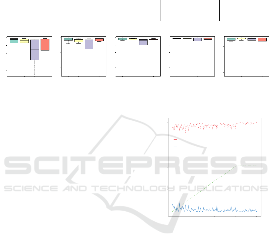
Table 3: Confusion matrix reporting the average number (and standard deviation σ) of true positives (TP), false positives (FP),
false negatives (FN), and true negatives (TN) of XCSR for the ten test data sets.
Actual class
Congested Free flowing Total
Prediction
Congested 248 (σ = 170) (TP) 5 (σ = 5) (FP) 253
Free flowing 12 (σ = 8) (FN) 1751 (σ = 170) (TN) 1763
Total 260 1756 2016
●
●
●
0.92 0.94 0.96 0.98 1.00
XCSR LaSVM LaSVM−I SDCA
Accuracy
(a) Accuracy.
● ●●
●
0.0 0.2 0.4 0.6 0.8 1.0
XCSR LaSVM LaSVM−I SDCA
Sensitivity
(b) Recall.
●
● ●●
●
●
0.0 0.2 0.4 0.6 0.8 1.0
XCSR LaSVM LaSVM−I SDCA
F−measure
(c) F-measure.
●
●
●
● ●●
●
●
0.0 0.2 0.4 0.6 0.8 1.0
XCSR LaSVM LaSVM−I SDCA
Precision
(d) Precision.
●
●
●
●
0.92 0.94 0.96 0.98 1.00
XCSR LaSVM LaSVM−I SDCA
Specificity
(e) Specificity.
Figure 5: The box plots show the statistical distribution of the average classification accuracy for XCSR, LASVM, LASVM-I,
and SDCA (left to right) considering occupancy and speed.
time steps. The points of each curve are the fraction
of the last 50 executions, averaged over ten runs. The
fraction correct is the percentage of correct classifi-
cations in the last 50 executions. The system error
is calculated as the absolute difference between the
actual reward and the system prediction P
a
of the se-
lected action, divided by the maximal reward (1000).
The population curve shows the average number of
micro classifiers normalised to the range of [0;1]. The
population size was roughly between 3400 and 5400.
Accordingly, we chose 6000 as the maximum number
of micro classifiers within the population. The curve
shows how the number of classifiers continuously in-
creases during the training phase. XCSR applied cov-
ering between 15 and 35 times (average: 24.4). The
number of GA executions ranges from 325 to 777 (av-
erage: 494.5), which translates to one GA execution
every 12th step during the training phase. Due to the
explorative behaviour of XCSR during training, the
fraction of correct classified instances and the system
error fluctuate more during this phase.
7 CONCLUSION
We applied the extended classifier system XCSR to
the task of detection of congestion patterns on inter-
states. The evaluation was done with real-world data
monitored by inductive loop detectors located in Min-
neapolis. In conclusion, it can be noted that XCSR
is able to evolve accurate classifiers, offering reliable
accuracy for the classification of traffic conditions.
Compared to three different types of support vector
machines, XCSR offers competitive performance.
0.00
0.25
0.50
0.75
1.00
0 2000 4000 6000 8000
Time step
Fraction correct, system error, population size (10 runs)
Fraction correct
Population size / 6000
System error / max. payoff
Figure 6: Average fraction correct, system error, and popu-
lation size for XCSR (feature vector: occupancy and speed).
Furthermore, XCSR is significantly faster in terms of
runtime for training and testing. In contrast to the
representation of support vectors, XCSR’s rule base
of classifiers of is easily interpretable by humans. We
plan to extend the binary classification problem by in-
troducing additional classes, such as tentative conges-
tion or continuing congestion. Instead of classifying
the current situation, XCSR can be adapted to pre-
dict the upcoming traffic conditions. Furthermore, we
want to investigate the performance of XCSR for ur-
ban congestion detection at intersections and sections,
following ideas from (Klejnowski, 2008).
Learning Classifier Systems for Road Traffic Congestion Detection
149

ACKNOWLEDGEMENT
The authors would like to thank Roman Sraj for his
contribution in the scope of his bachelor’s thesis.
REFERENCES
Alpaydın, E. (2008). Maschinelles Lernen. Oldenbourg.
Ben-Hur, A. and Weston, J. (2010). Data Mining Tech-
niques for the Life Sciences, chapter A User’s Guide
to Support Vector Machines, pages 223–239. Humana
Press.
Bordes, A., Ertekin, S., Weston, J., and Bottou, L. (2005).
Fast kernel classifiers with online and active learning.
Journal of Machine Learning Research, 6:1579–1619.
Brumback, T. E. (2009). A Mathematical Model for
Freeway Incident Detection and Characterization: A
Fuzzy Approach. PhD thesis, University of Alabama.
Bull, L., editor (2004). Applications of Learning Classifier
Systems. Springer.
Bull, L. and Kovacs, A. (2005). Foundations of Learn-
ing Classifier Systems, volume 183, chapter Founda-
tions of Learning Classifier Systems: An Introduction,
pages 1–17. Springer.
Bull, L., Sha’Aban, J., Tomlinson, A., Addison, J. D., and
Heydecker, B. (2004). Towards distributed adaptive
control for road traffic junction signals using learning
classifier systems. In Applications of Learning Clas-
sifier Systems, pages 276–299. Springer.
Butz, M. and Wilson, S. (2002). An algorithmic description
of XCS. Soft Computing - A Fusion of Foundations,
Methodologies and Applications, 6:144 – 153.
Deniz, O., Celikoglu, H. B., and Gurcanli, G. E. (2012).
Overview to some incident detection algorithms: A
comparative evaluation with istanbul freeway data.
Proc. of 12th Int. Conf. Reliability and Statistics in
Transportation and Communication, pages 274–284.
Diamantopoulos, T., Kehagias, D., Knig, F. G., and Tzo-
varas, D. (2014). Use of density-based cluster anal-
ysis and classification techniques for traffic conges-
tion prediction and visualisation. In Transp. Research
Arena Proceedings.
Ertekin, S., Bottou, L., and Giles, C. (2011). Nonconvex on-
line support vector machines. IEEE Trans. on Pattern
Analysis and Machine Intelligence, 33(2):368–381.
Holland, J. H. (1986). A mathematical framework for
studying learning in classifier systems. Phys. D, 2(1-
3):307–317.
Hsu, C.-W. and Lin, C.-J. (2002). A comparison of methods
for multiclass support vector machines. Trans. Neural
Networks, 13(2):415–425.
James, G., Witten, D., Hastie, T. J., and Tibshirani, R. J.
(2013). An Introduction to Statistical Learning.
Springer.
Klejnowski, L. (2008). Design and implementation of an
algorithm for the detection of disturbances in traffic
networks. Master’s thesis, University of Hannover,
Institute for Systems Engineering.
Lenz, B., Nobis, C., K
¨
ohler, K., Mehlin, M., Follmer,
R., Gruschwitz, D., Jesske, B., and Quandt, S.
(2010). Mobilit
¨
at in Deutschland 2008. DLR-
Forschungsbericht.
Liu, Q., Lu, J., Chen, S., and Zhao, K. (2014). Multiple
na
¨
ıve Bayes classifiers ensemble for traffic incident
detection. Mathematical Problems in Engineering,
2014.
Mahmassani, H. S., Haas, C., Zhou, S., and Peterman, J.
(1999). Evaluation of incident detection methodolo-
gies. Technical report, Center for Transportation Re-
search, University of Texas.
Ozbay, K. and Kachroo, P. (1999). Incident Management in
Intelligent Transportation Systems. Artech House ITS
library. Artech House.
Parkany, E. and Xie, P. C. (2005). A complete review of in-
cident detection algorithms & their deployment: What
works and what doesn’t. Technical report, Fall River,
MA: New England Transp. Consortium.
Picard, D., Thome, N., and Cord, M. (2013). Jkernelma-
chines: a simple framework for kernel machine. Jour-
nal of Machine Learning Research, 14(1):1417–1421.
Prothmann, H., Rochner, F., Tomforde, S., Branke, J.,
M
¨
uller-Schloer, C., and Schmeck, H. (2008). Organic
control of traffic lights. In Proc. of the 5th Int. Conf.
on Autonomic and Trusted Computing, volume 5060
of LNCS, pages 219–233. Springer.
Schrank, D., Eisele, B., and Lomax, T. (2012). 2012 Ur-
ban mobility report. Texas A&M Transp. Institute.
http://mobility.tamu.edu/ums/.
Shalev-Shwartz, S. and Zhang, T. (2013). Stochastic dual
coordinate ascent methods for regularized loss. Jour-
nal of Machine Learning Research, 14(1):567–599.
ˇ
Singliar, T. and Hauskrecht, M. (2006). Towards a learning
incident detection system. In Proc. of the Workshop
on Machine Learning for Surveillance and Event De-
tection at the 23
rd
Int. Conf. on Machine Learning.
Srinivasan, D., Jin, X., and Cheu, R. L. (2004). Evalua-
tion of adaptive neural network models for freeway
incident detection. In IEEE Transaction on Intelligent
Transp. Systems, volume 5, pages 1–11.
Wilson, S. (2000). Get real! xcs with continuous-valued
inputs. In Learning Classifier Systems, volume 1813
of LNCS, pages 209–219. Springer.
Yang, X., Sun, Z., and Sun, Y. (2004). A freeway traf-
fic incident detection algorithm based on neural net-
works. In Yin, F.-L., Wang, J., and Guo, C., editors,
Advances in Neural Networks - ISNN 2004, volume
3174 of LNCS, pages 912–919. Springer.
Zhang, K. and Xue, G. (2010). A real-time urban traffic de-
tection algorithm based on spatio-temporal OD matrix
in vehicular sensor network. Wireless Sensor Network,
2(9):668–674.
VEHITS 2017 - 3rd International Conference on Vehicle Technology and Intelligent Transport Systems
150
