
Two-level Approach for Scheduling Multiproduct Oil Distribution
Systems
Hossein Mostafaei
1,2
and Pedro M. Castro
1
1
Centro de Matemática Aplicações Fundamentais e Investigação Operacional,
Faculdade de Ciências, Universidade de Lisboa, 1749-016 Lisboa, Portugal
2
Department of Applied Mathematics, Azarbaijan Shahid Madani University, Tabriz, Iran
Keywords: Scheduling, Tree-like Structure, Decomposition Approach, Batch Sequencing.
Abstract: A core component of the oil supply chain is the distribution of products. Of the different types of distribution
modes used, transportation by pipeline is one of the safest and most cost-effective ways to connect large
supply sources to local distribution centers, where products are loaded into tanker trucks and delivered to
customers. This paper presents a two-level optimization approach for detailed scheduling of tree-like pipeline
systems with a unique refinery and several distribution centers. A mixed-integer linear programming (MILP)
formulation is tackled in each level, with the upper and lower level models providing the aggregate and
detailed pipeline schedules, respectively. Both models neither discretize time nor divide a pipeline segment
into packs of equal size. Solutions to two case studies, one using real-life industrial data, show significant
reductions in both operational cost and the CPU time with regards to previous two level approaches.
1 INTRODUCTION
In today’s competitive environment, supply chain
management is a major concern for companies and
has received growing attention in recent years. The
oil supply chain deals with a complex structure and
comprises many costly stages such as: oil exploration,
refining and product distribution, with transportation
costs already surpassing 400 billion dollars in the
early eighties (Bodin et al., 1983).
Different types of distribution modes are used in
the oil supply chain where the pipeline mode is the
most reliable and cost-effective way of transporting
high volumes of oil products between refineries
(upstream) and distribution centers nearby consumer
markets (downstream). Transportation scheduling of
petroleum products via pipelines is one of the most
challenging management problems with several
operational restrictions to be considered.
Pipelines convey a variety of oil derivatives such
as heating oil, motor gasoline, jet fuel, and liquefied
gas (one after the other). The products usually move
through several pipelines before reaching their final
destinations. Since there is not a physical barrier in
between products, some mixing occurs, producing a
contaminated product that is referred to as interface
material. An effective sequence of pipeline input and
output operations can considerably reduce pipeline
operating costs.
In recent years, several authors have applied
rigorous optimization tools to pipeline scheduling
problems, relying both on discrete- (Rejowski and
Pinto, 2003, 2004; Magatao et al., 2004; Herran et al.,
2010) and continuous-time MILP formulations
(Cafaro and Cerda, 2004; Castro, 2010; Cafaro and
Cerda, 2011; Mostafaei and Ghaffari, 2014;
Mostafaei et al. 2015a). They have generally
considered two operational plans for the pipeline
systems: aggregate and detailed, depending on the
way pipeline input and output operations are
performed. Aggregate plans define the optimal batch
sizes and the sequence of batch injections during the
time horizon, while detailed plans deal with
sequencing and timing of batch removals during a
pumping operation.
Mostafaei and co-workers (Ghaffari and
Mostafaei, 2015; Mostafaei et al., 2016, 2017)
developed continuous time MILP models to tackle the
operational planning of straight pipeline networks
that permits to achieve both the aggregate and the
detailed plans in single step. Compared to a two-level
approach developed by Cafaro et al. (Cafaro et al.
2012), they achieved better detailed schedules.
150
Mostafaei H. and Castro P.
Two-level Approach for Scheduling Multiproduct Oil Distribution Systems.
DOI: 10.5220/0006196501500159
In Proceedings of the 6th International Conference on Operations Research and Enterprise Systems (ICORES 2017), pages 150-159
ISBN: 978-989-758-218-9
Copyright
c
2017 by SCITEPRESS – Science and Technology Publications, Lda. All rights reserved
Cafaro and Cerda (2010) introduced a continuous
time MILP formulation for aggregate scheduling of
tree-like pipelines. Castro (2010) and Mostafaei et al.
(2015b) developed continuous time MILP
formulations to solve the detailed scheduling of the
same problem in a single step. However, the single
level optimization framework is computationally
expensive for large-scale problems. It is the main goal
of this paper to propose a computationally more
efficient approach relying on hierarchical
decomposition to generate the detailed schedule.
In previous two level approaches for straight
pipelines (Cafaro et al. 2011, 2012), each product
delivery operation in the lower level model should be
accomplished in the time interval determined in the
upper level model. Such a decision may not avoid
unnecessarily flow restarts if a depot is alternatingly
active in the aggregate schedule. This limitation is
also relaxed in this paper.
The rest of the paper is organized as follows:
Section 2 presents a brief description of the problem
under study. Section 3 builds a hierarchically
decomposition approach for the detailed scheduling
of the tree-like pipeline networks. The efficacy of the
proposed approach is tested using two case studies,
leading to the results in Section 4. The last section
puts forward the conclusions and sums up the paper.
2 PROBLEM STATEMENT
We deal with a short-term scheduling problem where
a tree-like pipeline must convey oil derivatives from
a single refinery to several distribution centers
(depots). Such a pipeline system consists of a trunk
line known as mainline (pipeline0) and several
secondary lines emerging from the mainline at
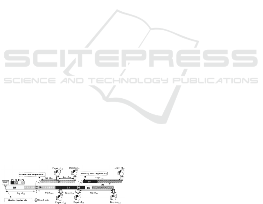
different sites (branch points). Figure 1 shows a tree-
like pipeline network with two secondary lines
(pipelines1,2). A pipeline segment ends with a
depot and/or a branch point. The secondary line 2 in
Figure 1 has two segments and two depots.
Figure 1: Tree-like pipeline system.
Batches of petroleum products pumped at the
refinery are diverted to mainline depots or/and
branched into secondary lines. The aim is to
determine the optimal batch input and output
operations in order to meet depot requirements at
minimum total cost subject to the following rules: (1)
pipeline segments remain full at any time; (2) each
pumping operation involves at most one batch
injection at the refinery (3) pipelines work in a single
flow direction, from left to right in the diagrams, (4)
the refinery should pump product into the mainline in
admissible injection rates; (5) in the detailed level, a
pumping operation can at most have one batch input
in each pipeline and in each depot whereas the
aggregate plan relaxes such assumption; (6) pipeline
segments should operate in acceptable flowrate
ranges, whereas in the aggregate level there are no
flowrate segment restrictions; (7) the valves of active
depots and segments remain open throughout the
pumping operation while they may be turned on/off
several times in the aggregate plan.
Given are the following: (i) the number of
products to be injected by the refinery (ii) the time
horizon length measured in hours (h), (iii) the 0-1
matrix of forbidden sequences between products, (iv)
capacity of pipeline segments measured in m
3
, (v)
volumetric coordinate of depots (m
3
), (vi) volumetric
coordinate of branch points (m
3
), (vii) pump rate at
refinery measured in m
3
/h, (viii) flowrate range in
pipeline segments (m
3
/h), (ix) maximum/ minimum
volume injected to each pipeline and diverted to
depots during each pumping operation (m
3
), (x)
product inventory at refinery and product demand at
depots (m
3
).
3 OPTIMIZATION MODEL
In this section, we present a two-level approach for
the detailed scheduling of tree-like pipelines. We will
sequentially solve the aggregate (upper level) and the
detailed (lower level) pipeline scheduling models
recently developed by Mostafaei et al. (2015b). The
aggregate model (referenced hereafter as the AP
model) will focus on batch input sequencing problem
whereas the detailed schedule (DP model) will
consider batch output sequencing problem in depots.
The approach uses the common sets defined in
Mostafaei et al (2015b): (1) ∈; pumping runs (2)
∈; pipelines, (3) ∈
; depots or segments of
pipeline , (4) ∈
,
,…
; batches to move
inside the pipeline network, (5)
; new batches to
be pumped into the mainline (
⊆), (6)
∪
; batches to move in pipeline , with
indicating the batches initially inside pipeline
and
denoting the batches to be transferred within
the planning horizon; (7) ∈; oil products, (8)
Two-level Approach for Scheduling Multiproduct Oil Distribution Systems
151

⊆
; batches to be diverted into depot
,
(9)
; product contained in old batch and (10)
;
non-empty old batches in secondary line . Note that
pipeline 0 is referred to as the mainline.
Two alternative objective functions will be
explored through the optimization approach. The
objective function of the AP model will minimize the
operational cost of pipeline, including pumping,
interface and backorder costs. The DP model will
reduce the pump operating and maintenance costs
subject to fully fulfilling all product deliveries
accomplished by the aggregated plan. As stated by
Hane and Ratliff (1995), most of the pipeline energy
consumption and the pump maintenance costs are
linked to flow restarts in idle pipeline segments and
consequently it is important to minimize the number
of pipeline segments where the flow is resumed or
stopped. Restarting the flow in a segment is
equivalent to saying that the segment is active
through the current pumping run but inactive during
the previous one. The opposite condition identifies
the stop of the pipeline segment.
Note that minimizing the number of flow
stoppages brings another economic benefit to the oil
industry since the size of the interface volume
between adjacent batches inside a segment tends to
increase while it stays inoperative. Future work will
involve enforcing pipeline segments to contain a
single product when they are inactive.
Here we present the AP and DP model. The list
of model entities can be found in Mostafaei et al.
(2015b).
3.1 Aggregate Level (AP)
3.1.1 Pumping Sequence
Let
be the start time of pumping run and
be
its duration. Pumping run can start if the previous
run 1 is completed. The length of all runs must
not surpass the length of planning horizon.
, ∀ ∈
2
(1)
∈
(2)
3.1.2 Tracing the Location of Batches
The continuous variable
,,
is used to track the
upper location of batch ∈
in pipeline at the end
of pumping run . This variable is equal to the volume
of batches
pursing batch ∈
at the end of
pumping run .
,,
,,
,
∈
:
∀ ∈
,∈,∈
(3)
3.1.3 Injecting Batches from the Refinery
Binary variable
,
is equal to one if batch ∈
is
receiving material from the refinery during pumping
run . During run , batch can receive material if the
lower coordinate of the batch (
,,
,,
)
touches the origin of the mainline at the end of
pumping run . If
,
1, a positive volume of batch
will be injected into the pipeline at the acceptable
pump rate belonging to the interval [
,
].
,
∈
1, ∀∈
(4)
,,
1
,
,∀ ∈
,
(5)
,
,,
,
,∀∈
, (6)
,,
∈
,,
∈
,∀
(7)
3.1.4 Product Allocation to Batches
Batch can at most convey a single product . Binary
variable
,
is used to allocate products to batches.
The volume of batch containing product pumped
from the refinery (
,,
) should be within a given
range. If it conveys a product, new batch ∈
will
be pumped into the mainline in one or more pumping
operations. Since each batch can convey a single
product, the volume of batch containing pumped
through run is equal to
,,
.
∑
,∈
1, ∀∈
(8)
,
∑
,,
,
,∀∈
,
(9)
∑
,∈
∑
,
,∀∈
∈
(10)
∑
,,
,,
,∀∈
,
(11)
3.1.5 Batch Removal at Depots
Through pumping run , a batch ∈
can be
discharged to depot
only if: (i) its upper coordinate
has reached the output facility of depot
,
at
time
and (ii) its lower coordinate has not
surpassed
,
. If binary variable
,,,
is equal to 1,
depot
receives a certain volume of batch ∈
(
,,,
) that is bounded by
,
,,
plus the material injected to batch from the origin of
pipeline during time interval [
;
].
ICORES 2017 - 6th International Conference on Operations Research and Enterprise Systems
152

,,
,
,
1
,,,
,
∀ ∈
,∈
,,
(12)
,,
,
,,,
,∀ ∈
,∈
,,
(13)
,
,,,
,,,
,
,,,
,
∀ ∈
,∈
,,
(14)
,
,,
,
,,
,,
,
1
,,,
,∀ ∈
,∈
,,
(15)
The volume of batch containing product
discharged to depot ∈
will be equal to
,,,
if batch conveys product , otherwise it will be zero.
∑
,,,,
∈
,,,
,∀∈
, ∈
,,
(16)
∑
,,,,∈
|
|
,
,
,∀∈
, ∈
,
(17)
3.1.6 Material Transferred to Secondary
Lines
Through pumping run , a batch in mainline can be
diverted to secondary line (
,,
1) if its upper
and lower coordinates satisfy
,,
,,
and
,,
. It means the
upper coordinate of batch has already reached
branch point and its lower coordinate has not
surpassed the coordinate of branch point (
).
If
,,
1, a portion of batch has entered
secondary line (
,,
.
,,
1
,,
,
∀ ∈
,,0
(18)
,,
,,
,∀∈
,,0
(19)
,,
,,
,,
,
∀ ∈
,,0
(20)
Let us define binary variable
,
to identify the
existence of batch in secondary line . For non-
empty old batch ∈
we have
,
1 and for
new batches ∈
:
,
∑
,,∈
|
|
,
,∀∈
,0
(21)
3.1.7 Interface and Forbidden Sequences
Batch 1
is injected into the mainline right
after
and consequently there will always be a
contamination product at their common boundary
which is referred to as interface. The volume of the
interface material depends on the specific products
and ’ is assumed to be given by parameter
,
.
If continuous variable
,,
,
is the interface
volume between batch and its successor in pipeline
conveying products and ′, we have the following
conditions for batches in the mainline and secondary
lines, where the domain of Eq. (23) is ,
∈
,
,,
∈,0:
,,,
,
,
,
,
1,
∀ ∈
,,
∈.
(22)
,,,
,
,
,
,
,
,
∑
,
,
2,
(23)
For quality reasons, some products should not
touch each other inside the pipeline. The next
equations prevent forbidden sequences in the
mainline and secondary lines.
,
,
1
,
,
∀ ∈
,,
∈
(24)
,
,
∑
,
,
,
,
3,∀∈
,
,,
∈,0
(25)
3.1.8 Size of Batch at the End of Run
At the end of pumping run, the size of batch in
pipeline can be obtained from its size at time
(
,,
) by adding the material that has entered
pipeline and subtracting the material transferred to
its depots and split lines. The next equations compute
the size of batch in the mainline and secondary lines.
,,
,,
,,
∑
,,,∈
∑
,,
,∀∈
,1
∈
(26)
,,
,,
,,
∑
,,,∈
,∀∈
,1,0.
(27)
3.1.9 Mass Balance
The total volume entering pipeline is equal to the
volume leaving the pipeline.
∑
,,∈
∑∑
,,,∈
∈
∑∑
,,∈
,∀∈
∈
(28)
∑
,,∈
∑∑
,,,
,
∈
∈
∀ ∈ , 0
(29)
3.1.10 Material Transferred from Batch to
Mainline’ Depots and Secondary
Lines
It is possible that during the execution of a pumping
run the volume of batch in the mainline can be taken
by multiple active depots and secondary lines. In this
case, the volume from batch to these depots and
lines is limited by the following equations.
∑
,,,
∈
:
,
∑
,,
∈:´
,,
,,
1
,,
,∀ ∈
,∈,∈
(30)
Two-level Approach for Scheduling Multiproduct Oil Distribution Systems
153

∑
,
,,
∈
∑
,,
:
,
,
,,
,,
1
,,,
, ∀ ∈
,∈,∈
(31)
3.1.11 Meeting Demand
The total volume of product unloaded to depot
during the planning horizon should be as large as
,,
, the demand of product at depot
.
Note that it is possible that some demand is not
satisfied within the planning horizon. Slack variable
,,
stands for the unsatisfied demand of
product at depot
.
∑∑
,,,,∈
∈
,,
,,
,∀∈,∈
,∈
(32)
3.1.12 Objective Function of Model AP
min
.
,,
∈∈
∈
,
.
,,
,
∈
∈∈∈
,,
.
,,
∈∈∈
3.2 Detailed Level (DP)
All constraints in model AP are part of model DP
except for the interface and forbidden sequence
constraints. The remaining constraints of model DP
model are listed below.
3.2.1 Feeding Depots and Secondary Lines
In detailed level, active depots must simultaneously
receive materials while inserting a new batch from the
refinery. Such a condition enforces active depot
to
receive material from batch during run if the upper
coordinate of the batch at the end of pumping run
1 (
,,
) has reached the volumetric coordinate
of the output facility of depot
,
. Moreover, the
lower coordinate of the batch should not surpass
,
at the end of pumping run . So Eqs. (12)-(13)
need to be changed by the following.
,,
,
,
1
,,,
,
∀ ∈
,∈
,,
(33)
,,
,
,,,
,∀∈
,∈
,,
(34)
Note that in detailed plan, the product delivery to
an active depot will be accomplished from a single
batch. This is not a model restriction but a practical
fact since delivery rates may vary with products.
Active secondary lines will also receive material from
a single batch in detailed level during each pumping
operation and therefore Eqs (18)-(19) should be
replaced by the following:
,,
1
,,
,
∀ ∈
,,0
(35)
,,
,,
,∀∈
,,0
(36)
Note that Eqs (33)-(36) increase the number of
pumping runs required to find the optimal solution,
which is detrimental for computational performance.
This is one of the reasons for applying two level
approaches for detailed pipeline schedule.
3.2.2 Activated and Stopped Volume
In detailed level, it is important to detect the pipeline
segments where the flow is resumed or stopped. To
this end, we need to determine the status of pipeline
segment in two consecutive runs. Binary variable
,,
takes the value of 1 if some material moves in
segment
through pumping run.Since the
pipeline network features a unique refinery,
segment1
will be active if segment
is
active, as imposed by Eq (37). The first segment of
mainline is active if the segment is receiving products
from the refinery (
∑
,
1
∈
), and vice versa.
The first segment of a secondary line will be active
when some material is transferred to this line from the
mainline (
∑
,,
1
∈
), and vice versa. On the
other hand, depot
will be idle if segment
is idle,
as imposed by Eq (40).
,,
,,
,∀∈
,,
(37)
,,
∑
,
,
∈
∀,
(38)
,,
∑
,,
,
∈
∀,,
(39)
∑
,,,∈
,,
,∀∈
,,
(40)
The model also needs to specify the status of the
mainline segments branching into secondary lines
(segments1
and 3
in Figure 1). Since
is the
volumetric coordinated of branch point and
,
is
the volume of segment
, we have:
,,
,,
,∀,,∈
|
,
(41)
To compute activated and stopped volumes, we
first need to determine the active volume of any
pipeline at the end of pumping run through
continuous variable
,
the volume from the
ICORES 2017 - 6th International Conference on Operations Research and Enterprise Systems
154
origin of to the end of furthest active segment
).
The active volume of a secondary line will be zero if
its first segment is idle.
,
,,
,,
.
,
,∀,,∈
(42)
,
,
,
1
,,
,,
,∀,, ∈
(43)
,
,,
,∀,0,
(44)
Activated volume of pipeline during run
(
,
) is the idle volume of the pipeline through
run 1, while the stopped volume (
,
) is the
active volume through run 1.
,
,
,
,∀∈,∈ (45)
,
,
,
,∀ ∈ , ∈ (46)
3.2.3 Flowrate in Pipeline Segment
Aggregate plans usually prevent enforcing flowrate
constraints on pipeline segments. These are important
since segments typically have different diameters.
The detailed plan, as an operational rule, should
consider flowrate restrictions, where
,
and
,
are minimum and maximum stream flowrates
in segment
. The flowrate in segment
can be
computed by the total volume of materials moving
along , divided by the pumping run length
.Eq
(47) enforces flowrate limitations in mainline
segment whereas Eq (48) restrains flowrates in
secondary segments.
,
1
,,
∑∑
,
,,
∈
∈
∑∑
,,∈
∈
,
,
,∀∈
,∈
(47)
,
1
,,
∑∑
,
,,
∈
∈
,
,∀∈
,∈
, 0
(48)
3.2.4 Objective Function of DP Model
min
,
,
∈∈
∙
,
∈∈
4 DECOMPOSITION APPROACH
The detailed scheduling of multi-branched tree
structure pipeline networks will become an
intractable problem even for short term horizons if all
decisions related to the pipeline input and output
operations are to be made in a single step. To find the
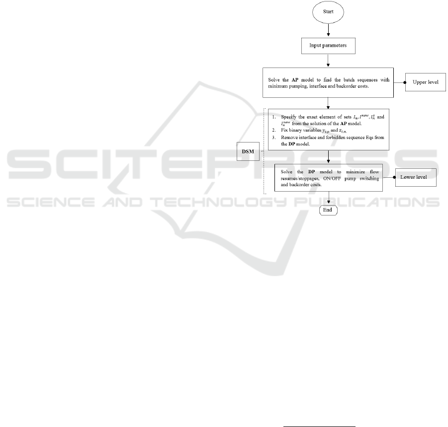
best detailed schedule in reasonable time, we first
solve the AP model to find the optimal batch
sequence in each pipeline at minimum interface,
pumping and backorder costs. The resulting solution
helps us to identify the exact elements of sets
,
,
and
,and consequently reduce the
constraints domain. Then, after fixing the binary
variables
,
and
,
and removing the interface and
forbidden constraints, we solve the DP model to meet
demand with minimum number of flow
resumes/stoppages and pumping operations. The
proposed decomposition procedure will hereafter be
called DSM and is depicted in Figure 2.
Figure 2: Proposed DSM framework.
4.1 Optimal Number of Pumping Runs
To solve both the upper and the lower models, we
should first guess the number of pumping operations
for each step. Like previous continuous time
approaches, we use an iterative procedure to find the
optimal number of pumping operations
|
|
to be
performed. In fact, searching for the optimal solution
can be extremely costly, but if the initial guess on the
number of pumping runs is accurate, no more than
two iterations are usually required. Since all
operations may not involve the maximum volume
(
), a simple expression for the number of
pumping operations of model AP can be:
∑∑∑
,,
||
Moreover, the number of pumping operations in
the model DP cannot be greater than the number of
Two-level Approach for Scheduling Multiproduct Oil Distribution Systems
155
product deliveries in model AP (PD
) and lower
than the number of pumping runs in AP:
||
|
|
PD
4.2 Previous Two Level Approaches
Cafaro and co-workers (2012) were the firsts to
develop a two-level approach for the detailed
scheduling of straight pipeline systems. In their
approach (hereafter CC), after finding the product
sequence with minimum pumping and interface costs,
they fix the aggregate batch sizes, the starting and
completion times of each pumping operation in AP,
and solve the second stage to generate a detailed
schedule. In fact, the start and end of pumping
operations for a batch injection in the lower level
must exactly comply with the start and end times
specified for that batch injection in the upper level
model. To this end, each product delivery in the lower
level model should be accomplished in the same time
interval performed in the upper level model. Since the
solution quality for the detailed scheduling problem
depends on the sequence of product deliveries, the
CC model does not usually find cost-effective
transportation plans.
5 COMPUTATIONAL RESULTS
Two case studies, one of them using industrial data,
were solved to validate the efficiency of the proposed
two level approach. The implementations were on an
Intel® Core(TM) i5-4210U (2.7 GHz) with 6 GB of
RAM, running Windows 7, 64-bit operating system
using GAMS/CPLEX 12.6 in parallel deterministic
mode (using up to 4 threads).
5.1 Example 1
This example deals with a small network and aims to
show how we select the elements of sets
,
,
and
in the lower level model (detailed schedule).
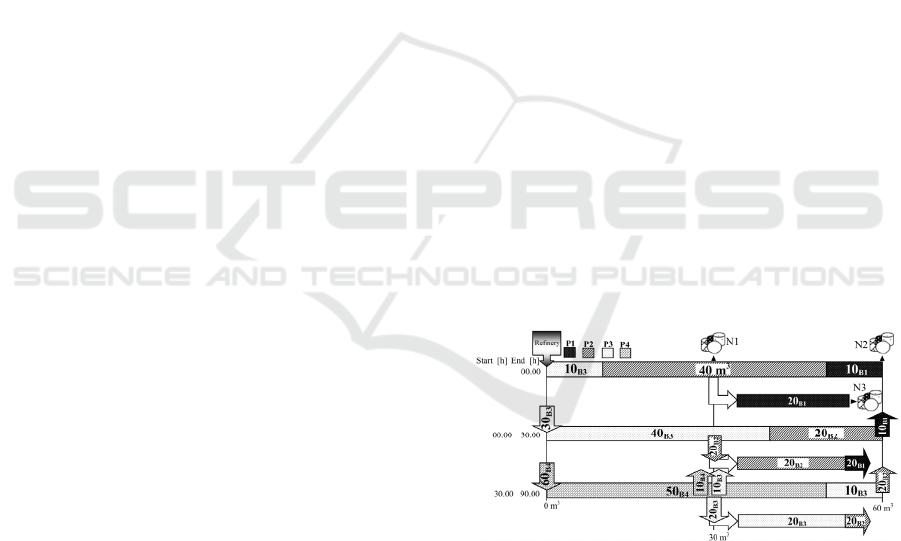
We assume that the aggregated transportation plan in
Figure 3 is already available. The pipeline topology
and its initial status at the start time of planning
horizon (time 0.00h) is depicted in the first row
of Figure 3. The flowrate in pipeline segments can
vary between 0.3 and 1.0 m
3
/h and the time horizon
has a length of 96 h (4 days). The maximum volume
input per pumping run is 60 m
3
while the minimum is
10 m
3
. The same condition holds for the minimum
and maximum batch size diverted to depots. The unit
stoppage cost is 0.4 in each segment.
The aggregate pipeline schedule contains two
pumping operations. The first operation takes place
from time 0.0 h to 30.0 h and involves increasing the
amount of product P3 in batch B3 and diverting 20 m
3
of B2 into the secondary line and 10 m
3
of batch B1
into depot N2. The second pumping operation from
30.0 to 90.0 h injects 60 m
3
of new batch B4 into the
mainline and the following delivery operations are
accomplished at depots: depot N1 receives from
batches B3 and B4; batch B2 goes to depots N2 and
N3.
To solve DP (lower level model) we should first
guess the number of pumping operations and specify
the exact elements of sets
,
,
and
. From
the aggregated plan, there are a total of 6 product
deliveries to depots and so 2
|
|
6. We will
start solving the problem with
|
|
2and keep
increasing
|
|
until no improvement is found in
the objective function.
From the solution obtained from the AP model,
we can now refine the elements of sets
,
,
and
and reduce the domain of the constraints. It
can be observed from Figure 3 that only new batch
B4 is injected into the mainline. There are three old
batches B1, B2 and B3 and so
B4,B3,B2,B1.
Two new batches B2 and B3 are injected into the
secondary line (pipeline1) and so
B3,B2.
There is only one old batch B1 inside the secondary
line and so
B1,B2,B3
. Depot N1 only
receives product from batches B3 and B4 and so
B3,B4. Similarly, we have
B1,B2
.
Figure 3: Aggregate pipeline schedule for Example 1.
Figure 4 shows the optimal detailed schedule for
Example 1 using DSM. It contains 4 batch injections
at the refinery and 7 product deliveries to depots. The
injection of batch B3 (and batch B4) from the refinery
is now accomplished through a sequence of two short
pumping runs. There is only one segment stoppage
during 4 days that happens in the secondary line
during time interval [60.00, 90.00].
ICORES 2017 - 6th International Conference on Operations Research and Enterprise Systems
156
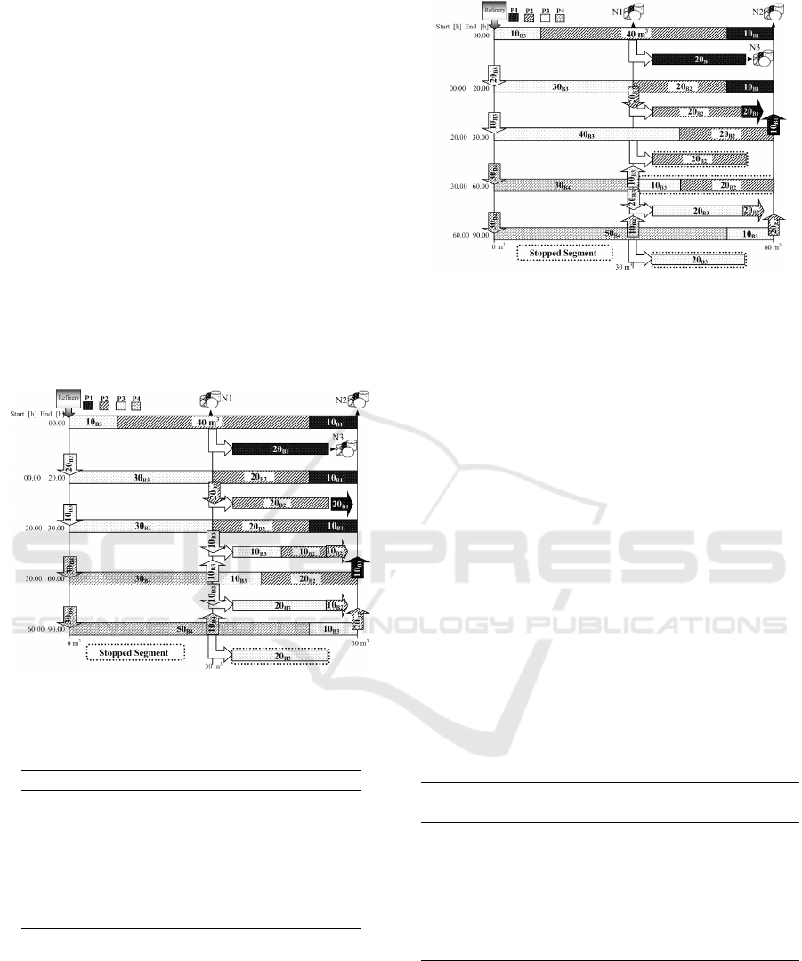
Figure 5 shows the optimal pipeline schedule for
Example 1 using CC. Like DSM, 4 batch injections
should be accomplished to fully satisfy the given
demands. Note that 10 m
3
of batch B1 are being
discharged into depot N2 during time interval [0.00,
30.00] of the aggregate plan of Figure 3. This depot
should extract the same amount of material during
time interval [0.00, 30.00] of the detailed plan. In
contrast, it remains inactive in DSM (see Figure 4).
The aggregate transportation plan enforces depot N2
to be idle during [30.00, 60.00] and to be active
during [60.00, 90.00] in CC. Such a change in the
status of depot N2 leads to a stoppage in the last
segment during the third pumping operation.
Superfluous flow shutdowns can also be observed in
the secondary line that are due to the change in the
status of depot N3 that alternatingly becomes active
and idle.
Figure 4: Detailed schedule for Example 1 using DSM.
Table 1: Computational results for Example 1.
DSM CC
# Pumping runs 4 4
# Constraints 646 646
# Binary vars 90 90
#Continuous vars 285 285
CPUs 0.47 0.42
Stop vol (m
3
) 20 70
Obj. Fun
a
($) 8 28
a
Both DSM and CC only minimize pipeline stoppage volumes.
Table 1 gives the computational results of
Example 1 for the CC, DSM approaches. Though the
number of pumping operations is the same, the
stopped volume of the pipeline in the proposed
approach decreases from 70 to 20 m
3
. Such a lower
shutdown volume in pipeline leads to cost savings of
71.42 %.
Figure 5: Detailed schedule for Example 1 using CC.
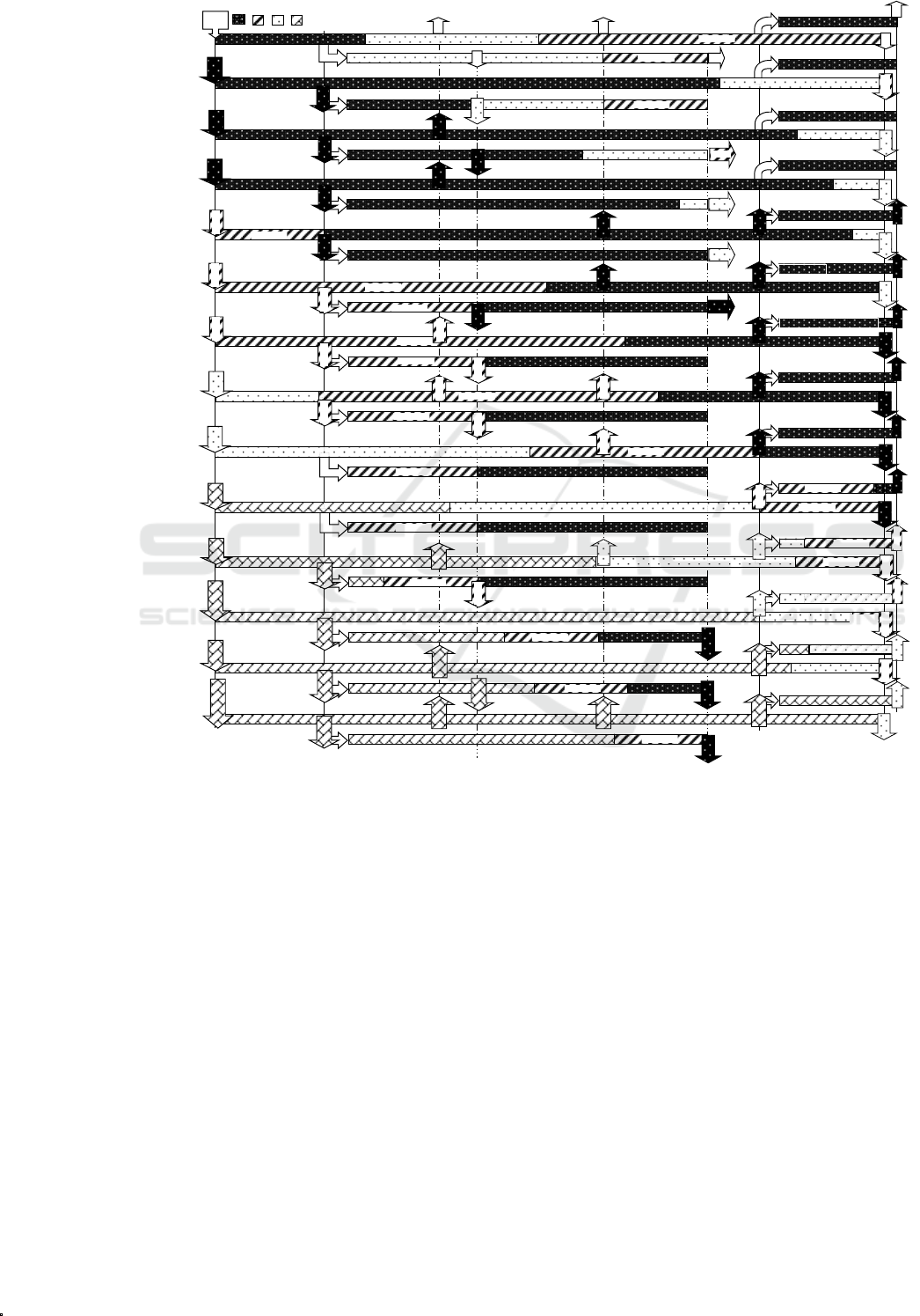
5.2 Example 2 (Real-Life Case Study)
Here we consider a large-scale real-world example
from Mostafaei et al. (2015a), involving an Iranian
tree-like pipeline with a refinery, a mainline, two
secondary lines and six depots (check first row of
Figure 6). The first secondary line with two depots
starts 3000 m
3
away from the mainline’ origin while
the other secondary line (single depot) leaves the
mainline after 15000 m
3
. Batches of four products
(P1-P4) should be conveyed and it is forbidden for P1
to touch P4. The product injection rate can vary
between 300 and 800 m
3
/h, and the time horizon has
a total length of 192 h. In both aggregated and
detailed levels, at most 13000 m
3
of each product can
be injected into the mainline during each operation.
Other data for this example, together with the
aggregate transportation plan, can be found in
Mostafaei et al. (2015b).
Table 2: Computational results for Example 2.
DSM CC Mostafaei et al.
(2015b)
# Pumping runs 13 22 12
# Constraints 5076 9090 5864
# Binary vars 671 1381 782
#Continuous vars 2500 6281 3714
CPUs 64.4 412.60 468.23
Restart vol (m
3
) 39200 118400 39200
Obj. Fun
a
($) 15680 47360 15680
a
Both DSM and CC only minimize pipeline restart volumes.
Figure 6 shows the optimal detailed schedule for
Example 2 using DSM. It contains 13 pumping
operations and 50 product deliveries to depots. Model
size and computational requirements for Example 2
are reported in Table 2.
Two-level Approach for Scheduling Multiproduct Oil Distribution Systems
157
12600
4100 4900 m
3
3800
9600
Ref
N1 N2
N3 N4
N6
N5
6000 2400
13700 4900
3000 3000
2400
3800
3800
3800
500
3000
3000
9600
13000
16137.5
4562.5
2437.5
2462.5
6000
5400 3000
3600
2400
3700
16831.25 1768.75
693.75
2368.75
7768.75
631.25 2368.75
637.5
3000
3000
8800
11800
14500 1100
668.75
631.25
8400
1200
631.25
3300
500
500
8800
9800
1100
1600 2200
1100
3000
1700
3600
1100
1300
9600
3200
3200
500
3000
3000
3000
3000
3000
5400
5400
5400
5400
5400
5400
3400
1700
500
3300
1700
6800
1300
2920
2920
9880
5800
500
500
3800
500
500
500
920
5580
8500 6500 3600
3800
1270
1270
930
3380
6500
6500 8500 3600
2900
900
2900
2900
3600
7200
1000
1000 2000
1000
10600
2100
5300 2700
2900900
900
900
900
2300
7157.143
2757.143
15000
3757.143
2000
2000
2000
2757.143
2400
3800
2900
1500
2900
9600
16200
2400
4957.143
2642.857
1442.85
1200
1200
1200 2600
12002600
2400
1200
2400
18600
6400
1200
1442.857
1442.857
11542.857
3100
2600
4800
1200
2000
00.00
Start[h] End [h]
00.00 19.20
19.20 35.45
35.45 40.07
40.07 44.02
44.02 55.02
55.02 68.02
68.02 71.67
71.67 80.97
80.97 93.97
93.97 102.97
102.97 112.64
112.64 124.64
124.64 136.07
P1
P2 P3 P4
3800
Figure 6: Detailed schedule for Example 2 using DSM.
Three interesting conclusions can be derived from
the results. The first, is that the optimal detailed
schedule by the CC approach involves 22 pump
operations against 13 by DSM. The second, is that the
solution CPU time has been reduced by a factor of 7
with regards to CC. The third, is that the objective
function value for DSM is 66.89 % less expensive
than the one for CC. This is due to substantial
reductions on shutdown volumes. Compared with the
single level approach of Mostafaei et al (2015b), the
proposed DSM approach finds the same solution in a
lower CPU time.
6 CONCLUSIONS
This paper presented a novel optimization framework
for the detailed scheduling of treelike pipeline
networks. The network consists of a refinery, a trunk
line, a set of split lines and multiple depots. A
computationally efficient two-level approach based
on a pair of MILP models has been presented. In the
upper level, the optimal sequence of batches in each
pipeline is found while the lower level deals with the
detailed plan that computes the optimal sequence of
batch removals at depots. Through the solution of two
ICORES 2017 - 6th International Conference on Operations Research and Enterprise Systems
158

case studies, we showed that the proposed model is
more flexible than previous hierarchical approaches
and is able to solve large scale problems in reasonable
time. Future work will involve applying the proposed
method for multi-level tree pipeline networks, with
intermediate due dates on demands over long-term
horizons.
ACKNOWLEDGMENTS
Financial support from Fundação para a Ciência e
Tecnologia through the Investigador FCT 2013
program and project UID/MAT/04561/2013.
REFERENCES
Bodin, L., Golden, B., Assad, A. and Ball, M., 1983.
Routing and scheduling of vehicles and crews. The
State of the Art. Computers &Operations Research, 10
(2), 62.
Cafaro VG., Cafaro DC., Mendéz CA., Cerdá J., 2011.
Detailed scheduling of operations in single-source
refined products pipelines. Industrial & Engineering
Chemistry Research, 50: 6240-6259.
Cafaro, D. C., Cerdá, J., 2004. Optimal scheduling of
multiproduct pipeline systems using a non-discrete
MILP formulation. Computers & Chemical
Engineering, 28, 2053-2068.
Cafaro, D. C., Cerdá, J., 2011. A rigorous mathematical
formulation for the scheduling of tree-structure pipeline
networks. Industrial & Engineering Chemistry
Research, 50, 5064-5085.
Cafaro, V. G., Cafaro, D. C., Mendéz, C. A., Cerdá, J.,
2012. Detailed scheduling of single-source pipelines
with simultaneous deliveries to multiple offtake
stations. Industrial & Engineering Chemistry Research,
51, 6145-6165.
Castro, P. M., 2010. Optimal scheduling of pipeline
systems with a resource-task network continuous-time
formulation. Industrial & Engineering Chemistry
Research, 49, 11491-11505.
Ghaffari-Hadigheh, A., Mostafaei, H., 2015. On the
scheduling of real world multiproduct pipelines with
simultaneous delivery. Optimization and Engineering,
16, 571-604.
Hane, C. A., Ratliff, H. D., 1995. Sequencing inputs to
multi-commodity pipelines. Annals of Operations
Research, 57, 73-101.
Herran, A., de la Cruz, J. M., de Andres, B., 2010.
Mathematical model for planning transportation of
multiple petroleum products in a multi-pipeline system.
Computers & Chemical Engineering, 34, 401-413.
Magatao, L., Arruda, L. V. R., Neves, F. A., 2004. A mixed
integer programming approach for scheduling
commodities in a pipeline. Computers & Chemical
Engineering, 28, 171-185.
Mostafaei, H., Alipouri, Y., Shokri, J., 2015. A mixed-
integer linear programming for scheduling a multi-
product pipeline with dual-purpose terminals.
Computational and Applied Mathematics, 34, 979-
1007.
Mostafaei, H., Castro, P. M., Ghaffari-Hadigheh, A.,
2015b. A novel monolithic MILP framework for lot-
sizing and scheduling of multiproduct treelike pipeline
networks. Industrial & Engineering Chemistry
Research, 54, 9202–9221.
Mostafaei, H., Castro, P. M., Ghaffari-Hadigheh, A., 2016.
Short-term scheduling of multiple source pipelines with
simultaneous injections and deliveries. Computers &
Operations Research, 73, 27-42.
Mostafaei, H., Castro, P.M., 2017. Continuous-time
scheduling formulation for straight pipelines. AIChE J.
doi: 10.1002/aic.15563.
Mostafaei, H., Ghaffari-Hadigheh, A., 2014. A general
modeling framework for the long-term scheduling of
multiproduct pipelines with delivery constraints.
Industrial & Engineering Chemistry Research, 53,
7029-7042.
Rejowski, R., Pinto, J. M., 2003. Scheduling of a
multiproduct pipeline system. Computers & Chemical
Engineering, 27, 1229–1246.
Rejowski, R., Pinto, J. M., 2004. Efficient MILP
formulations and valid cuts for multiproduct pipeline
scheduling. Computers & Chemical Engineering, 28,
1511–1528.
Two-level Approach for Scheduling Multiproduct Oil Distribution Systems
159
