
Optimization Techniques for Routing Design Problems over Wireless
Sensor Networks: A Short Tutorial
Ahmed Ibrahim
1,2
and Attahiru Alfa
1,3
1
Department of Electrical and Computer Engineering, University of Manitoba, Winnipeg, MB, Canada
2
Faculty of Engineering and Applied Sciences, Memorial University of Newfoundland, St. John’s, NL A1B 3X5, Canada
3
Department of Electrical, Electronic and Computer Engineering, University of Pretoria, Pretoria 0002, South Africa
Keywords:
Wireless Sensor Networks, Design, Routing, Optimization, Tutorial.
Abstract:
This paper is intended to serve as an overview of, and mostly a short tutorial to illustrate, the optimization
techniques used in several different key design problems that have been considered in the literature of routing
over wireless sensor networks. For each routing design problem, a key paper that implements optimization
techniques is selected, and for each we present the formulation techniques and the solution methods imple-
mented. We observed that good formulation is the key to fully exploiting the features of the techniques. Hence
we focus on presenting the formulation techniques, to facilitate the use of “on the shelf” efficient algorithms
in the operations research literature. This we believe will help researchers in better understanding the issues
and how to improve further on solution techniques.
1 INTRODUCTION
As the technology evolves, the wireless sensors man-
ufactured become technically more powerful and
economically viable. In wireless sensor networks
(WSNs) each node consists basically of units for
sensing, processing, radio transmission, position find-
ing and sometimes mobilizers (Al-Karaki and Kamal,
2004), (Papadopoulos et al., 2016). These sensors
measure desired phenomenal conditions in their sur-
roundings and digitize them to process the received
signals to reveal some characteristics of the condi-
tions in the surrounding area. A large number of
these sensors can be networked in many applications
that require unattended operations, hence producing
a WSN. In general, the sensor nodes in a wireless
sensor network WSN sense and gather data from sur-
rounding environment and route it to one or more
sinks, to perform more intensive processing. The
number of applications for WSNs is large, many of
these are in the fields of weather monitoring, surveil-
lance, health care, etc. More fields are deploying
WSNs as their reliability, performance and capabili-
ties keep getting even better and wider.
In many applications, replacement of damaged
or energy depleted nodes is not possible. Moreover
planned nodal placement may not be a possible thing
to do. Therefore, two of the main requirements for
WSNs to operate reliably are to consume the min-
imum amount of energy to prolong the network’s
life time, and to be able to self organize themselves
when the network topology changes. Other require-
ments (e.g limited delay, good signal to noise ratio,
etc.) are usually application specific. Moreover, there
are differences in the nature of WSNs. For exam-
ple, there could be WSNs with either rechargeable or
non-rechargeable sensor batteries, either single sink
WSNs or multiple sink WSNs, which could either
be immobile or mobile. Depending on these differ-
ent variants of WSNs, different types of applications
and the traffic types they handle, different design con-
siderations will need to be taken into account. Opti-
mization techniques that have been in the operations
research (OR) literature for almost a century provide
a rich reservoir of different types and classes of opti-
mization problems that have been studied extensively.
For these, different solution techniques are available
that have experienced development over the years un-
til they have reached to a mature level in which their
computational and storage performance have been ex-
tensively tested and assessed. Among these are the
different variants of Lagrangian relaxation (Fisher,
2004), dual decomposition methods (Sontag et al.,
2011) column generation (Desaulniers et al., 2006)
and many others. One of the benefits of dual de-
composition techniques is that an optimization prob-
156
Ibrahim A. and Alfa A.
Optimization Techniques for Routing Design Problems over Wireless Sensor Networks: A Short Tutorial.
DOI: 10.5220/0006188201560167
In Proceedings of the 6th International Conference on Sensor Networks (SENSORNETS 2017), pages 156-167
ISBN: 421065/17
Copyright
c
2017 by SCITEPRESS – Science and Technology Publications, Lda. All rights reserved

lem can be decomposed and each node given a local
part of it hence enabling a distributed solution scheme
rather than a centralized one.
We believe that in order to exploit the full strength
of the extensive tools in the optimization literature,
good formulation is necessary to reduce the design
problem to one of the classical optimization prob-
lems for which those well studied solution techniques
could be used. In this paper, such techniques are il-
lustrated for the different routing design problems in
WSNs, for which we have selected seven papers to
discuss. We summarize the various routing design
problems and the corresponding optimization tech-
niques used in Table 1 whose columns show:
1. the design problem,
2. the initial optimization problem formulations,
3. the design objective,
4. the centralized/distributed possible algorithmic
implementation to solve the initial formulations,
5. any reformulations performed,
6. solution algorithms that were proposed,
7. whether the proposed algorithms are distributed
or centralized,
8. the nature of the solution that could be obtained,
whether it is suboptimal or global optimal,
9. the convergence speed or computational complex-
ity of the solution algorithms.
A section is dedicated for each routing problem in
which we give the system model and the design objec-
tives, the problem formulation and solution methods
considered in those papers. The notation in each sec-
tion is restricted to that section only. We use the same
notation used by the original papers to make it easier
for the reader to connect the paper with the originals
we consider here.
2 ROUTING FOR MULTI-HOP
WSNS WITH A SINGLE
IMMOBILE SINK
A multi-hop wireless sensor network was considered
in (Madan and Lall, 2006) that focuses on computing
multi-hop routes from each node to a single immo-
bile sink such that the network lifetime is maximized.
The lifetime in (Madan and Lall, 2006) was defined
as the time at which the first node runs out of energy.
Each node can generate information due to its sens-
ing capabilities and relay packets from other nodes to
the sink node. The nodes’ battery energies are limited
and adjustments of transmission powers for each node
is possible depending on the distance between nodes.
2.1 Optimization Problem Formulation
The initial formulation given in (Madan and Lall,
2006) is a max-min non-linear program (NLP) where
the objective function maximizes the minimum of all
lifetimes across the nodes in the network. The life
time of each node is defined as the quotient of the ini-
tial battery energy of the node to the sum of expended
energies on each of the node’s outgoing flows. The
decision variables are continuous and represent the
transmission rates r
i j
for a node i to node j. The con-
straint set, is a linear equality set of conservation of
flow constraints for all the nodes in the network. They
simply state that the difference between the outgoing
flows from each node and its incoming flows should
strictly be equal to the data generated by the node it-
self.
To make the problem easier, the minimum term in
the objective function is replaced by an auxiliary con-
tinuous variable which is upper bound constrained by
the lifetime of all sensor nodes. This adds more struc-
ture to the problem making it a quadratically con-
strained program. Further reformulation techniques
were used to reduce it to an equivalent linear program
which introduced an auxiliary continuous variable q.
2.2 Solution Methods
Two solution methods were provided in (Madan and
Lall, 2006), one is a partially distributed scheme and
the other is fully distributed. For both, the Lagrangian
for the objective function is obtained. The dual func-
tion is the minimum Lagrangian function where the
minimizers are the primal variables of the problem
which are r
i j
and q. The primal decision variables ap-
pear in separate additive terms in the Lagrangian and
hence the dual function can be evaluated separately at
each node.
The resulting linear primal objective function gets
modified, by squaring it, to an equivalent strictly
convex function plus a strictly convex regularization
term. Also a loose upper bound is imposed on the
auxiliary variable so that all decision variables have
bound constraints that form a bounded polyhedron.
These two modifications ensure that the dual function
is differentiable and hence enables the use of the sub-
gradient algorithm with guarantee that it converges to
the solution of the strictly convexified primal prob-
lem. The dual function for the strictly convexified
problem is still separable in the primal variables. In
each iteration of the subgradient algorithm, a box con-
Optimization Techniques for Routing Design Problems over Wireless Sensor Networks: A Short Tutorial
157
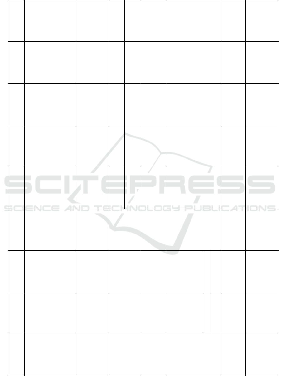
Table 1: Summary of the covered WSN routing problems and the corresponding optimization techniques.
Routing Design As-
pect
Classification of Initial
Problem Formulation
Objective
Initial problem formu-
lation: Centralized /
Distributed?
Classification of Refor-
mulated Problem
Solution Method
Implemented solution
scheme for the prob-
lem : Centralized /Dis-
tributed?
Nature of Solution
Convergence Speed /
Complexity
Routing for a WSN
Multi-hop with Single
Immobile Sink (Madan
and Lall, 2006)
bilinear quadratically
constrained program
Maximizes the shortest
lifetime across all nodes
Centralized
1. reformulated to
linear program
2. reformulated
to strictly con-
vex quadratic
program
Dual Decomposition +
subgradient algorithm
1. Partially dis-
tributed for
linear program
reformulation
2. Fully distributed
for the strictly
convex quadratic
program reformu-
lation
Global Optimal
1. Partially dis-
tributed algorithm
: around 600 sub-
radient iterations
to converge
2. Fully distributed
algorithm :
around 3500 sub-
gradient iterations
to converge
Routing in a delay-
tolerant WSN to a
Single Mobile Sink
(Yun et al., 2013)
Quadratically Con-
strained Program
Maximize the number
of cycles made by mo-
bile sink
Centralized Linear program
Lagrangian relax-
ation +subgradient
algorithm, greedy al-
gorithm for fractional
knapsack problems+
trivial heuristic for
box constrained linear
program
Decentralized algorithm
Good Suboptimal .
Global Solution is also
attainable in a long time
Good suboptimal in few
iterations (100-200) and
global after too many it-
erations.
Joint routing, power
and bandwidth alloca-
tion in FDMA WSNs
(Leinonen et al., 2013)
Non-strictly convex
non-linear constrained
program
Minimize the aggregate
power for all network
links
Centralized
Convex non-linear
global consensus prob-
lem
Augmented Lagrangian
+Alternating direction
method of multipliers
Distributed among
nodes
Global optimal
Fast, converged in 21 it-
erations of the ADMM
algorithm
Strictly convex non-
linear program (using
proximal regularization)
Dual decomposition and
projected subgradient
algorithm
Distributed among
nodes and decomposed
in protocol layers
Global optimal
Slower than ADMM,
converges in 133 iter-
ations of th projected
subgradient algorithm
Energy and route allo-
cation from multiple
source to multiple des-
tination in rechargeable
WSNs (Chen et al.,
2012)
Complicated Convex
NLP
Maximize Aggregate
node utilities
Centralized
Decomposed to two eas-
ier strictly convex sub-
problems by decoupling
the time component
Dual decomposition
+subgradient algorithm
used in a heuristic
scheme
Distributed
suboptimal in finite time
but optimal in infinite
time
Too slow, took 5000
minutes to reach the best
suboptimal solution in
the simulations done in
(Chen et al., 2012)
Account for uncertain-
ties in the distance be-
tween sensor nodes (Ye
and Ordonez, 2008)
Linear Program
Aggregate transmission
and reception normal-
ized energies
N/A
• Polyhedral uncer-
tainty set: yields
Linear Program
• Ellipsoidal uncer-
tainty set: yields a
second order cone
program (SOCP)
Interior point methods,
CPLEX solver was used
to solve the problem
N/A Global optimum
Can be solved in poly-
nomial time
Linear Program
Maximize the transmit-
ted data to the sink
Bilinear Constrained
Program
Maximize the network
lifetime
Joint Routing and
Scheduling in WSNs
with Multiple Sinks and
Different Sink Location
Possibilities (Gu et al.,
2011)
Non -Linear and non-
deterministic (due to the
integration function)
Maximize the network
lifetime
Centralized
Non-Linear Quadrat-
ically constrained
Program
Column Generation
Method
Centralized Global Optimal
Too quick for small
problems (less than one
second and 6 iterations)
but unknown for large
problems
Joint Routing and
TDMA scheduling for
delay sensitive under-
water acoustic WSNs
(Ponnavaikko et al.,
2013)
NLP with general unde-
termined nonlinear term
in the objective function
Minimize the transmis-
sion energy
Centralized
Mixed Integer Linear
Program
Not stated, an MILP
solver is assumed to
have been used
Centralized
Global optimal to the
MILP but is subopti-
mal to the original NLP
problem
Depends on the desired
approximation error.
Expected to be fast for
large approximation
errors but slow for
small approximation
errors, hence there is a
trade-off.
SENSORNETS 2017 - 6th International Conference on Sensor Networks
158

strained single variable quadratic and convex problem
gets solved. The obtained values of the primal vari-
ables are used to calculate the values of the dual vari-
ables in the next iteration by the subgradient formulas.
At a given iteration k , the values of the dual vari-
ables needed to solve for the flow transmission rate
variables r
k
i j
of a node are locally available to the sen-
sor node. The transmission rates of a node’s links
could hence be computed at that node only without
the need of any communication with other nodes.
The calculation of the problem’s auxiliary variable
q
k
however, needs all the values dual variable values
from all the nodes in the network to be transmitted to
the node responsible its computation. The auxiliary
variable values obtained in every iteration hence need
to be broadcasted to all the nodes as they are needed
for the subgradient calculation in the following itera-
tion.
For the i
th
element of the subgradient to be com-
puted at node i for iteration k, it needs the rate vari-
ables values at iteration r
k
ji
for all its neighbors in the
set N
i
to be transmitted to it. Therefore, each node
has to broadcast its r
k
i j
values to its neighbors. Then,
using those, the value of q
k
received from a broadcast
and the locally calculated r
k
i j
, the i
th
element of the
subgradient gets calculated at node i. The values of
the new dual variables are calculated locally at each
node.
Since every node contributes in the computation
of the primal variables, dual variables and the subgra-
dient at each iteration, the algorithm is therefore like
a distributed one. However, the algorithm is not fully
distributed since at iteration k, node i still needs other
calculated variables from other nodes.
Another algorithm was proposed in (Madan and
Lall, 2006) that is fully distributed. The linear pro-
gram is transformed into a strictly convex quadratic
optimization problem by introducing a separate aux-
iliary variable q for each node i. Then, instead of
maximizing the primal objective function in a sin-
gle variable q
2
as in the problem, the sum of q
2
i
is maximized. By enforcing an equality constraint
q
i
= q
j
,∀i ∈ V,∀ j ∈ N
i
(where V is the set of nodes
and N
i
is the set of neighbors of i) which guarantees
that for any feasible solution the objective function is
just
|
V
|
q
2
which yields the same set of feasible solu-
tions and the same optimal solution. This change en-
ables the dual problem to be decomposed to separate
node local problems which each node can solve in-
dependently with only the exchange of dual variables
with its neighbors.
3 ROUTING IN SINGLE MOBILE
SINK
A WSN with a mobile sink was considered in (Yun
et al., 2013). Each node can postpone data transmis-
sion until the sink is at the most favorable position
to extend the lifetime of the network. The problem
is to find how long the sink should stay at potential
stops and how buffered data could be routed to the
sink when it stops taking into account a maximum
delay toleration. A distributed algorithm was used in
which the problem is decomposed to smaller decision
problems and each can be solved by a sensor node.
Only local information from the neighbors is needed
by each node.
The network was modeled as a directed graph
where the cost of each arc is proportional to the dis-
tance between the nodes of that edge. The sink must
complete each of its tours through all available sink
positions and back to the initial position within the
maximum tolerable delay. The problem was found to
be equivalent to maximizing the number of sink tours
T within the tolerable delay for which the life time is
the total number sink cycle durations. The sink does
not have to visit all the locations in an optimal solu-
tion. Also, when it is at a particular position , only a
set of nodes R
l
⊆ N (where N is the set of nodes in
the network) can transmit data via multi-hops to the
sink. The other nodes not in R
l
do not transmit to the
sink when it is at l and buffer their data instead. The
set R
l
is chosen depending on experimental trials. For
each location l, there is a graph G
l
=
N ∪
{
l
}
,A
l
where A
l
=
{
(i, j) ∈ A|i ∈ R
l
∪
{
l
}}
and A is the set
of arcs in the main directed graph that represents the
network.
An expanded graph G
exp
that comprises all the
graphs G
l
and a vertex node s, that represents the sink
, is constructed. The details of the construction are
given in (Yun et al., 2013).
3.1 Optimization Problem Formulation
The optimization problem was initially formulated as
a quadratically constrained program QCP. The de-
cision variables x
(l)
i j
represent the data flow between
two nodes i and j with the sink at position l, y
(l)
i
rep-
resentthe amount of buffered data at node i just as the
sink leaves location l and T represents the number of
cycles the mobile sink makes. All the decision vari-
ables are continuous.The objective function maxi-
mizes the number of cycles the mobile sink makes i.e.
max
T,x
(l)
i j
,y
(l)
i j
T . This is a linear objective function in one
Optimization Techniques for Routing Design Problems over Wireless Sensor Networks: A Short Tutorial
159

continuous variable.
There are two constraint sets. A linear equal-
ity constraint set that combine the transmission flows
and buffered data for all possible sink locations to
enforce conservation of flow constraints which guar-
antee that the total incoming flows for node i plus
the buffered data is equal to the outgoing flows. A
quadratic constraint set that guarantees that all the en-
ergy expended due to data transmission on the links
for all possible sink positions is within the available
node’s battery remaining energy. It was given by
∑
L
l=1
∑
j∈N
l
(i)
e
(l)
i j
x
(l)
i j
T ≤ E
i
, ∀i ∈ N where e
(l)
i j
is
the energy spent per unit data on the link (i, j) when
the sink is at position l and E
i
is the available energy
for node i and E
i
is the available battery energy for
node i.
The problem was reformulated to a linear pro-
gram by minimizing the reciprocal of the number of
sink cycles and substituting that reciprocal with an-
other continuous variable z = 1/T . The quadratic
constraint now becomes
∑
L
l=1
∑
j∈N
l
(i)
e
(l)
i j
x
(l)
i j
≤
zE
i
, ∀i ∈ N in the new formulation.
3.2 Solution Method
Lagrangian relaxation was used to dualize the set of
flow equality constraints. The Lagrangian dual func-
tion is then minimized with respect to the primal vari-
ables z, x and y where the vectors x and y comprise
of the variables x
(l)
i j
and y
(l)
i
respectively. The La-
grangian dual optimization problem minimizes the
Lagrangian dual function subject to the energy con-
straint for each node.
The Lagrangian dual optimization problem is de-
composed into two subproblems S1 and S2. The sub-
problem S1 consists of a linear objective function in
the primal vector y and decision variable bound con-
straints on the variables y
(l)
i
. Subproblem S2 con-
sists of a linear objective function in z and the vector
x. The constraints for S2 are the energy constraints
∑
L
l=1
∑
j∈N
l
(i)
e
(l)
i j
x
(l)
i j
≤ zE
i
, ∀i ∈ N and variable
bound constraints. One subproblem was reduced to
a linear box constrained problem whose minimum
value was obtained in a distributed manner by each
node by setting its corresponding buffering variable
y
(l)
i
to their upper bound if their respective coefficient
in the objective function of the subproblem is negative
and zero otherwise. The second subproblem was re-
duced to multiple fractional knapsack problems that
could be solved separately by each node (hence de-
centralized approach) in polynomial time. The sub-
gradient algorithm was used to evaluate the values of
the dual variables on an iteration by iteration basis.
4 JOINT ROUTING, POWER AND
BANDWIDTH ALLOCATION
In (Leinonen et al., 2013) a frequency division multi-
ple access (FDMA) based single-immobile-sink WSN
was considered. The objective is to jointly allocate
data flows and bandwidth for the network links in or-
der to minimize the total transmission power in the
WSN. Flat fading was assumed which makes the link
rates dependent only on the power levels and the
bandwidth of the link irrespective of frequency de-
pendent gains. Each sensor i has a limited total power
P and a total preallocated bandwidth W
i
. The power
and bandwidth allocated to the sensor’s links l ∈ O (i)
should satisfy
∑
l∈O(i)
p
l
≤ P and
∑
l∈O(i)
w
l
≤ W ∀i
where p
l
and w
l
are the power and bandwidth on link
l respectively.
Each node allocates disjoint and continuous fre-
quency bands to its outgoing links. All nodes are
assumed to have a maximum communication range,
therefore a link between two nodes exists only if both
are within the communication range of each other.
The flow on a link cannot exceed Shannon ’s capacity
of the link.
4.1 Optimization Problem Formulation
All the decision variables are continuous non-
negative variables. There are three sets, one set of
variables is for the power values on the links p
l
, the
second is for the flow capacities on the links f
l
and the
third is for the amounts bandwidth spectrum allocated
to the links in the network w
l
. The objective function
is a linear function in the aggregate link powers i.e.
∑
l∈L
p
l
(where L is the set of links). There are four
constraint sets,
1. a linear equality constraint set in the flow vari-
ables f
l
for the conservation of data rate flows.
These guarantee that for every node the difference
between the out-going flows and the sum of the
in-going flows is strictly equal to the rate of data
generated by each node t
i
,
2. a convex non-linear constraint set that guarantees
that the flows on each link are upper bounded
by the Shannon capacity of the link. These con-
straints are function in both the powers on the
links p
l
and the bandwidths allocated to the links
w
l
and are given as, f
l
≤ c
l
(p
l
,w
l
) ∀l ∈ L,
3. a linear constraint set in the power variables of the
links that guarantees that for each node the aggre-
gate transmission power on all its links does not
exceed sensor’s battery power, i.e.
∑
l∈O(i)
p
l
≤
SENSORNETS 2017 - 6th International Conference on Sensor Networks
160

P,∀i ∈ S where S is the set of nodes and O (i) is
the set of links for node i,
4. a linear constraint set in the bandwidth variables
that guarantee that the sum of bandwidths allo-
cated on all the links of every node does not ex-
ceed the nodes’ pre-allocated bandwidth W , i.e.
∑
l∈O(i)
w
l
≤ W , ∀i ∈ S .
The objective function and all constraints but the
flow conservation constraint set can be considered an
independent local problem for each node to solve.
Consensus reformulation is used by introducing lo-
cal copies
ˆ
f
il
of the associated global flow variables
for each node.The local variables were interpreted in
(Leinonen et al., 2013) as the node’s opinion about
the corresponding global flow variables. By carry-
ing out the following modifications to the formula-
tion, the problem becomes a global consensus prob-
lem where except for the consensus constraints, the
rest of the modified constraints are local to each node.
1.
ˆ
f
il
≤ c
l
(p
l
,w
l
) ∀l ∈ L, ∀i ∈ S, l ∈ O (i)
2.
∑
l∈L(i)
a
il
ˆ
f
il
= r
i,
∀i ∈ S
3.
ˆ
f
il
= f
l
∀i ∈ S,l ∈ L (i) , which represent the con-
sensus constraints.
where a
il
∈
{
−1,0,1
}
is a constant whose possible
values describe the incidence of a graph edge on a
node, and L (i) denotes the set of links connected to
sensor node i and r
i
is the source rate for node i.
4.2 Solution Method
The augmented Lagrangian for the problem’s global
consensus reformulation is obtained with respect to
the consensus constraints. An L
2
norm penalty term
is added to regularize the non-differentiable optimiza-
tion function so that convergence is possible due to
the non-differentiable nature in the objective func-
tion. The alternating direction multiplier method
(ADMM) method is used to solvetheglobal consensus
formulation. It consists of a sequence of optimization
phases over the primal variables followed by a gradi-
ent method that updates the dual variables.
In each node, phase 1 minimizes the augmented
Lagrangian over the node local variables power, band-
width and flow variables p
i
,w
i
and
ˆ
f ). The second
phase minimizes over the global flow variable ( f
i
) for
each node i. Then, the dual variable corresponding
to each link for the node is updated with the constant
step size ρ. Phase 1 problem is a quadratic convex op-
timization problem in the local resource variables and
the local flow variables. Interior-point methods were
used by the authors to solve it. The phase 2 prob-
lem was manipulated algebraically to give the simple
form:
f
k
l
=
(
1
2
ˆ
f
k
tran(l)
+
ˆ
f
k
rec(l)
, f or all but the sink node
ˆ
f
k
tran(l)
, f or the sink node
(1)
where k is the iteration index, tran (l) and rec(l) are
the transmitting and receiving nodes on the link l re-
spectively. Thus, the global flow variables are ob-
tained at each iteration k by averaging out the cor-
responding updated local variables.
The only information that needs to be shared
among the nodes are the local flow variables. These
have to be broadcasted by each node to its neighbors.
The communications overhead therefore depends on
the network density, rather than the number of nodes.
5 RECHARGEABLE WSNS WITH
MULTIPLE SOURCES AND
DESTINATIONS
In (Chen et al., 2012), a rechargeable WSN whose
batteries’ replenishment profile is unknown a priori
is considered. Routing and energy allocation are
performed such that the aggregate utility functions
for the sensors is to be maximized with low com-
plexity. It was shown that the problem can be for-
mulated as a standard convex optimization problem
with energy and routing constraints. However, the
solution requires centralized control and full knowl-
edge of replenishment profiles in the future, which
may not be available in practice. Therefore, a low-
complexity heuristic solution was developed that is
asymptotically optimal and can be approximated by
a distributed algorithm.
The following are the main elements of the sys-
tem model in (Chen et al., 2012) are as follows. The
system is time slotted system with finite number of
slots and the battery of each sensor is assumed to
have an infinite rechargeable capacity. Multiple sens-
ing sources and multiple destination nodes are consid-
ered. A utility function that reflects the "satisfaction"
of the node is associated with each source node when
it transmits at an average data rate ˆx
s
(t) that is equal
to the aggregate amount of data from that source to a
particular destination over all time slots averaged over
the duration of the frame. It is defined generally to be
concave monotonically increasing in the average data
rate of the source node.
5.1 Problem Formulation
A formulation that maximizes the sum of general util-
ities of all sensor nodes was formulated as a convex
Optimization Techniques for Routing Design Problems over Wireless Sensor Networks: A Short Tutorial
161

NLP. All decision variables are continuous variables.
There are three sets of those, w
i j
(t) is the amount of
data on the outgoing link (i, j) for time slot t, x
s
(t)
is the amount of data delivered from source f
s
to the
destination d
s
, e
s
(t) represents the amount of energy
expended by a node. The objective function is the
sum of individual node utilities where each of these,
U
s
1
T
∑
T
t=1
x
s
(t)
, is a function of the amount of data
delivered from source node f
s
to destination node d
s
in all T time slots over possibly multiple hops and
multiple paths. Each utility function is assumed to be
a continuous non-linear concave function. There are
two constraint sets, the first is conservation of flow
constraint sets, which are linear constraints in w
i j
(t)
and x
s
(t). The second ensures that the sum of flows
emanating from a node i belongs to the set Λ
i
of the
different amounts of data in different time slots un-
der a given replenishment profile vector
−→
r
i
. For any
data vector in Λ
i
, there exists an energy vector e
n
that
achieves that amount of data for a given modulation
and coding scheme. The set Λ
i
was proved to be con-
vex in works earlier to (Chen et al., 2012).
5.2 Solution Method
A heuristic method named DualNet was proposed that
obtains an infeasible upper bound and a feasible lower
bound and iteratively solves the problem until it con-
verges to the optimal solution infinity. First an up-
per bound was obtained on the value of the objective
function at the optimal solution of the problem after
a long period of time (theoretically infinity). The so-
lution that gives the upper bound is obtained by an
infeasible energy allocation i.e. energy allocation that
is higher than the average replenishment rate. The en-
ergy allocation (and hence the routing solution) are
the same over all time slots and is more than the av-
erage replenishment rate, yielding infeasiblity. Using
the energy allocation obtained, a routing sub-problem
that is strictly convex and computationally easier than
the original problem is obtained because of the decou-
pling of the time component. This requires solving
the problem every time slot.
The lower bound solution is obtained by assign-
ing a feasible energy value in each time slot for each
node. The energy assignment for a node is the min-
imum of either the average harvested energy or the
available battery energy (including the instantaneous
replenishment for a given time slot). This assignment
is done by each node on its own and hence is a dis-
tributed energy assignment. Using the energy assign-
ment values the routing subproblem that obtains the
lower bound, is again a similar routing subproblem to
that of the upper bound subproblem.
Dual decomposition was used to solve the pro-
blem which enabled a distributed implementation of
the scheme. Each source node solves two prob-
lems, one to determine the amount of data to inject
in the network at a given time slot t, x
s
(t), the other
subproblem to determine the routes and their flows,
w
i j
(t). All the nodes that are not sources of data, and
only responsible for relaying data over multiple hops,
solve the routing problem only. The dual variables are
computed using the subgradient algorithm.
6 ROUTING WITH DISTANCE
UNCERTAINTIES
Optimization models were considered in (Ye and Or-
donez, 2008) for WSNs subject to distance uncer-
tainty for three different objectives, 1) minimizing the
energy consumed, 2)maximizing the data extracted
and 3) maximizing the network lifetime. Robust opti-
mization was used to take into account the uncertainty
present. In a robust optimization model the uncer-
tainty is represented by considering that the uncertain
parameters belong to a bounded, convex uncertainty
set. A robust solution is the one with best worst case
objective over this set. It was shown in (Ye and Or-
donez, 2008) that solving for the robust solution in
these problems is just as difficult as solving for the
problem without uncertainty. The computational ex-
periments in (Ye and Ordonez, 2008) showed that, as
the uncertainty increases, a robust solution provides a
significant improvement in worst case performance at
the expense of a small loss in optimality when com-
pared to the optimal solution of a fixed scenario.
6.1 Problem Statement and Design
Objectives
For the three different types of problems, energy con-
sumption was considered. The transmission and re-
ception energy for each node is accounted for after
normalizing with respect to the radio energy dissi-
pation of the transmitter and receiver circuits. The
expression for the total normalized energy has two
components. One for the normalized received energy
which is equivalent to the number of received bytes,
i.e.
∑
j|( j,i)∈A
f
ji
, and one for the the normalized trans-
mitted energy, which is equivalent to the number of
transmitted bytes times a linear function in the trans-
mission distance, i.e.
∑
j|( j,i)∈A
f
ji
1 + βd
2
i j
, where
• A is the set of nodes in the network,
• f
i j
is the number of transmitted bytes from node j
to node i.
SENSORNETS 2017 - 6th International Conference on Sensor Networks
162

• d
i j
is the distance from node i to node j and β is a
constant depending on transceiver parameters.
6.2 Formulations for the Three
Problems
A brief description of each of the three different op-
timization problems that were given in (Ye and Or-
donez, 2008) is as follows:
1. The Minimum Energy Problem: The decision
variables are the continuous variables f
i j
. The
objective function is a continuous linear objec-
tive function in f
i j
which is the sum of the trans-
mission and reception normalized energies of all
nodes in the network. The objective is to min-
imize that aggregate energy function. There are
two constraint sets, the first constraint set en-
forces a minimum data transmission requirement
constraint that requires the aggregate data trans-
mitted from all nodes to the sink node, to be
greater than a minimum number of bytes. The
second and third constraint sets are conservation
of flow constraints that require the difference be-
tween the amount of data bytes transmitted and
received by a node to be less than the available
data bytes at the node and greater than zero.
2. The Maximum Data Extraction Problem: The de-
cision variables are also f
i j
. The objective func-
tion maximizes the data transmitted to the sink
node. It was given as the sum of data bytes f
i j
transmitted from each node i to the sink node n+1
on the arcs (i, n + 1). It is a continuous linear ob-
jective function. As for the constraint sets, be-
sides the conservation of flow in the Minimum
Energy Problem, there is a set of energy limita-
tion constraints for each node, that guarantees that
the the sum of transmitted and received energy for
each node does not exceed the available energy of
the node, i.e.
∑
j|(i, j)∈A
f
i j
1 + βd
2
i j
+
∑
j|(i, j)∈A
f
i j
≤ E
i
∀i ∈ N.
(2)
Note that in (Ye and Ordonez, 2008), the energy
is normalized such that E
i
is the number of bytes
that could be transmitted with the available en-
ergy and the left hand side of the constraint is
the amount of bytes transmitted for an expended
amount of energy. All constraints are linear and
hence the problem is a linear program ignoring
the uncertainties.
3. Maximum Lifetime Problem: The objective func-
tion: maximize the lifetime T of the network
which is defined as the lifetime of the first
sensor whose battery gets depleted, i.e. T =
min
{
T
1
,T
2
,...,T
n
}
. The constraints are Conser-
vation of flow typical to those in Minimum En-
ergy Problem, in addition a quadratic constraint
with bilinear terms that guarantees that the energy
expended by transmission of a node i does not ex-
ceed its available energy, this is given by:
T
∑
j|( j,i)∈A
f
ji
+
∑
j|( j,i)∈A
f
ji
1 + βd
2
i j
!
≤ E
i
(3)
This gives a quadratically constrained program,
which is transformed to a linear program by sub-
stituting the variable T in the problem with q =
1/T and minimizing the objective function in-
stead of maximizing it.
6.3 Accounting for Uncertainties in the
Formulation
According to (Ye and Ordonez, 2008) a robust solu-
tion for an optimization problem under uncertainty
is defined as the solution that has the best objective
value in its worst case uncertainty scenario. For an
optimization problem under uncertainty with decision
vector x and uncertainty vector parameter u, the robust
solution is defined as:
min
x
n
max
u
f (x,u) : g(x , u) ≤ 0 ∀u ∈ U
o
(4)
which is equivalent to :
min
x,γ
γ : g(x, u) ≤ 0, f (x, u) ≤ γ ∀u ∈ U (5)
where U is a closed convex uncertainty set. Ac-
cording to (Ye and Ordonez, 2008), the complex-
ity of solving the robust counterpart of an optimiza-
tion problem is equivalent to solving the deterministic
problem for many problems. Moreover the increase in
size of the problem is polynomial in the deterministic
problem dimensions.
For the three optimization problems, the distance
parameter was considered as the uncertainty parame-
ter and hence in (Ye and Ordonez, 2008) was made
to belong to the uncertainty set U. The set U defines
distance vectors that are within a certain distance from
a given estimate of the distance vector between nodes.
The paper presented two general convex sets for the
uncertainty region, these are polyhedral sets and el-
lipsoidal sets. For both types of uncertainty sets, the
three deterministic optimization problems that were
considered were formulated to their robust counter-
parts. The type of optimization problems obtained for
the three cases are as follows:
Optimization Techniques for Routing Design Problems over Wireless Sensor Networks: A Short Tutorial
163

a. Polyhedral uncertainty sets: Using LP duality, it
was shown that optimization problem remains as a
linear program with additional variables and con-
straints.
b. Ellipsoidal sets: Using a known closed form so-
lution for an embedded ellipsoidal optimization
subproblem with respect to the uncertainty vari-
ables, the robust optimization problem becomes a
conic convex problem that can be solved by in-
terior point methods in polynomial time. With a
simple reformulation trick of replacing the conic
component in the objective function with an up-
per bound linear component and bringing in the
conic component in the constraint set, the problem
can be rewritten as a second order cone program
(SOCP).
Furthermore, simulation results showing the ob-
tained objective function values for the robust and de-
terministic solutions were also provided in (Ye and
Ordonez, 2008). The robust solutions were obtained
for different degrees of uncertainty, while the deter-
ministic solutions assumed complete certainty. The
results showed the average and standard deviations of
the objective functions over 100 random experiments.
The deterministic solution gave a higher average ob-
jective function value compared to the robust solution
while the standard deviation of the uncertainty level
of the robust objective value was closer to its mean
values as compared to the deterministic objective val-
ues.
7 WSNS WITH MULTIPLE SINKS
HAVING DIFFERENT
LOCATION POSSIBILITIES
In (Gu et al., 2011) scheduling and routing of data to
multiple sinks having multiple position possibilities
are considered. The objective is to maximize the net-
work lifetime which is defined in (Gu et al., 2011) as
the time elapsed since the launch of the network till
the instant a living node cannot find a route to send
its data to the sinks due to many dead nodes. The au-
thors propose two formulations for the same problem
which they state that they are equivalent but do not
provide a proof for that.
7.1 Initial Problem Formulation: Time
based Formulation
The first formulation considered the time to be contin-
uous and an independent variable based upon which
all decision variables are dependent. It was named as
time-based formulation and was considered very hard
to tackle. A brief description of this formulation is as
follows:
• Decision variables: T is a continuous variable that
represents the network’s lifetime, g
i j
(t) is a con-
tinuous variable that represents the data rate on the
link from node i to node j at a given time t, g
io
(t)
is a continuous variable that represents the data
rate from node i to one of the possible sinks’ posi-
tions o at a given time t, x
s,o
(t) is a binary variable
that is set only when sink s resides in position o.
• Objective function: is to maximize the lifetime of
the network which is given as max
T,g
i j
(t),g
io
(t),x
so
(t)
T ,
• Constraint Sets: The constraints sets of the initial
formulation are explained below:
1. Constraint set 1: is a linear constraint set in
the binary variables x
s,o
(t) that guarantees that
a possible position o at t can get occupied by
no more than one sink node, this is given as
∑
s∈V
s
x
s,o
(t) ≤ 1, ∀o ∈ V
o
, where V
s
and V
o
are
the sets of sink nodes and possible sink posi-
tions respectively.
2. Constraint set 2: is a linear constraint set in the
binary variables x
s,o
(t) that guarantees that sink
s at time t can only reside in one location, this
is given as
∑
o∈V
o
x
s,o
(t) ≤ 1, ∀s ∈ V
s
.
3. Constraint set 3: linear conservation of flow
equality constraints in the flow variables g
i, j
(t)
and g
i,o
(t).
4. Constraint set 4: variable upper bounds on the
flow variables g
i, j
(t) from node to node links
that represent the link capacity.
5. Constraint set 5: a mixed integer linear con-
straint in the variables g
i,o
(t) and x
s,o
(t) that
impose link capacity on the flows from node
i to the possible sink location o if any sink is
assigned to that location, otherwise the flow is
enforced to be zero. The constraint is g
i,o
(t) ≤
C
i,o
.
∑
s∈V
s
x
s,o
(t) ∀l
i,o
where C
i,o
is the capacity
of the link l
i,o
.
6. Constraint set 6: An energy constraint for each
sensor i ∈ S which is an integration of linear
terms with respect to the time parameter t with
the decision variable T in the upper limit of the
integral.
7. Constraint set 7: non-negativity constraints on
all the decision variables.
SENSORNETS 2017 - 6th International Conference on Sensor Networks
164

7.2 Reformulation: Pattern based
Formulation
As was mentioned for the time-based formulation in
(Gu et al., 2011), the life-time variable T is connected
to the rest of the variables through the energy con-
straint by integrating over time. This constraint com-
plicates the problem and makes it difficult to solve
according to (Gu et al., 2011). Therefore a reformula-
tion was performed to obtain an easier problem which
discretized the time parameter into different durations
to give an easier problem which has no integration in
any of the constraints. For each duration, a placement
pattern can be assigned such that the amount of en-
ergy expended over all time durations is within the
initial available energy level of each node. The life
time of the network is hence equivalent to the aggre-
gate discretized time durations. In each time duration,
an assigned pattern should satisfy all the constraint
sets that were explained for the time-based formula-
tion. The energy constraint in a given time duration
t
p
for placement pattern p becomes a linear constraint
in the flow variables g
p
i, j
and g
p
i,o
. The elements of the
reformulated problem are (Gu et al., 2011):
• Decision variables:
1. the continuous variables t
p
which represent the
assigned time durations for the possible pat-
terns p,
2. continuous variables e
p
i
for the energy con-
sumption rate for node i in pattern p for all
nodes and patterns,
3. binary decision variables x
p
s,o
tell whether sink
node s is assigned to location o in the pattern
placement p for all nodes, sinks and patterns
4. continuous variables g
p
i,o
for the data rate flow
from node i to the sink position o in pattern p
for all nodes, sinks and patterns,
5. continuous variables g
p
i, j
for the data flow rate
on the link between the nodes i and j in pattern
p for all nodes and patterns,
• Objective function: Maximizes the aggregate du-
rations assigned to the patterns which in (Gu et al.,
2011), was stated to be equivalent to the lifetime
of the network, i.e. max T =
∑
p∈P
t
p
.
• Constraint sets: The same constraint sets for the
time-based formulation should be satisfied for
each pattern, the energy constraints however are
replaced by two constraint sets for each pattern,
one is linear and the other is bilinear quadratic.
The linear one is an equality constraint that links
the energy expended by the node in a given place-
ment pattern with the flow variables g
p
i, j
and g
p
i,o
.
The bilinear constraint set guarantees that all the
energies expended by every node in all pattern du-
rations do not exceed their initial battery energies.
7.3 Solution Method: Column
Generation Method
Since the possible patterns are too large to enumer-
ate, the column generation method was used in (Gu
et al., 2011) for solving the following master problem
obtained from the pattern-based formulation in (Gu
et al., 2011):
max
t
p
,e
p
i
T =
∑
p∈P
t
p
:
∑
p∈P
e
p
i
t
p
≤ E
i
∀i ∈V, e
p
i
,t
p
≥ 0 ∀ i, p
(6)
where V
s
is the set of sink nodes , V
o
is the set of sink
possible locations and V is the set of non-sink sensor
nodes.
Different patterns correspond to columns in (Gu
et al., 2011). The master problem is given by the
pattern-based formulation except for e
p
i
which is
treated as a constant. It is hence a linear programming
problem. The subproblem that determines which col-
umn to enter solves for the pattern that would give
the maximum increase in the objective function of the
master problem. If the objective function of the mas-
ter problem cannot be improved any further then the
optimal solution has been reached.
An initial set of patterns P
0
can be obtained by ran-
dom assignment of sinks to locations and using short-
est path Dijkstra’s algorithm for routing to the nearest
sink. The master problem is then solved and the corre-
sponding optimal dual variables are obtained to sub-
stitute in the objective function of the sub-problem,
which is given by a linear equation representing the
reduced cost of the master problem. The reduced cost
is function in e
p
i
, which is the only variable in the ob-
jective function of the subproblem. The constraint
sets for the subproblems are linear conservation of
flow constraints and flow capacity constraints on all
links including the links to possible sink locations.
8 DELAY-SENSITIVE ROUTING
IN UNDERWATER WSNS
Underwater acoustic WSNs (UWA-SNs) were con-
sidered in (Ponnavaikko et al., 2013). The propaga-
tion delay in UWA-SNs is five times larger than in RF
networks which has a non-negligible impact on the
performance of UWA-SNs especially since they cover
much larger areas (square kilometers) unlike the RF
WSNs. In (Ponnavaikko et al., 2013) the propagation
Optimization Techniques for Routing Design Problems over Wireless Sensor Networks: A Short Tutorial
165

delay sensitivity was accounted for in optimizing en-
ergy for routing purposes. According to the authors
of (Ponnavaikko et al., 2013), this was not consid-
ered before their work due to the added complexity it
brings in.
The sensor nodes are immobile and have relay-
ing capabilities that enables the WSN to use multi-
hop communication to convey a packet from any sen-
sor to a sink node. Slotted synchronous time division
multiple access (TDMA) was the type of medium ac-
cess control (MAC) scheme considered. The objec-
tive was to design an offline routing scheme to pre-
calculate the number of slots per link and the amount
of data to be transmitted on each link while factoring
in the large propagation delays of water acoustic sig-
nals. The routing scheme proposed in (Ponnavaikko
et al., 2013) was named Delay-constrained Energy-
constrained Routing (DER).
8.1 Initial Problem Formulation
The initial problem formulation in (Ponnavaikko
et al., 2013) is a nonlinear program (NLP) with a non-
deterministic generic objective function in the deci-
sion variables and linear sets of constraints. A brief
explanation of the formulation is given as follows:
• Decision variables:
1. the number of bits transmitted on each link
(W
i j
),
2. the transmission time allocated for each link
(∆
i j
).
• Objective function: is the sum of all energy con-
sumed on all links in the network. It contains
P
W
i j
∆
i j
which is a non-deterministic general term
that is function in the number of bits W
i j
to be
transmitted on each link and the allocated transmit
time ∆
i j
. This term represents power consumption
which is dependent on the modulation/channel
coding schemes used for transmission.
• Constraint sets:
1. A linear delay constraint , that takes into ac-
count the propagation delay of each link and the
transmission delay that is inherent in the allo-
cated transmission time. The total delays on all
links from the source sensor nodes to the sink
should not exceed a maximum allowable delay
T , that was given by
∑
N−1
i=1
∑
j∈ψ
i
(∆
i j
+ τ
i j
) ≤ T
where τ
i j
is the propagation delay of link (i, j)
and ψ
i
is the set of neighbors for node i.
2. A linear conservation of flow set of constraints
for every node that guarantees that difference
between incoming and outgoing data is equal
to the amount of data generated by the sensor
node, that is
∑
j∈ψ
i
W
i j
−
∑
j∈ψ
0
i
W
i j
= r
i
T where
r
i
is the data generation rate of node i.
8.2 Reformulation
The objective function is linearized by substituting
P
W
i j
∆
i j
∆
i j
, the non-linear term, with an auxiliary
variable ε
i j
and adding to the constraint set the fol-
lowing equality constraint:
log (ε
i j
) = P
L
log (W
i j
− log (∆
i j
)) + log (∆
i j
) (7)
as well as the following equality constraint that con-
nects the logarithm of the transmission rate with the
number of bits transmitted and the transmission time
allocated:
log (R
i j
) = log (W
i j
) − log (∆
i j
) (8)
where
• ε
i j
is a new variable that represents the energy ex-
pended for transmission of data on link (i, j).
• P
L
is a constant that represents the relation be-
tween the logarithm of the power on a particular
link with respect to the logarithm of the transmis-
sion rate on that link.
The non-linear inequality constraints (7) and (8) are
piecewise linearized by Special Ordered Set type 2
(SOS2) variables and break points giving a Mixed In-
teger Linear Program (MILP). To approximate the
logarithms of the energy , power and the allocated
time on each link, five vectors of k SOS2 variables
were introduced where k is such that the approxima-
tion error is within 1%. Not more than two adjacent
SOS2 variables can be non-zero otherwise the rest of
the variables are enforced to zeros.
8.3 The Solution Method
There was no mention for the solution algorithm to
be deployed by the network. A generic MILP solver
is believed to be used for the numerical experiments,
however it was not stated which procedures of those
should be implemented in the network entity respon-
sible for the routing implementation.
9 CONCLUSIONS
In this paper we explored and illustrated how differ-
ent optimization techniques were used in solving dif-
ferent routing problems over WSNs. We explained
the formulations that were done for these problems,
SENSORNETS 2017 - 6th International Conference on Sensor Networks
166

classified them according to their types and explained
the solution techniques used. A common set of con-
straints in most routing problems turns out to be the
conservation of flow constraint sets. Mostly the ob-
jective is to minimize the energy consumption or
maximize the network lifetime. We explained how
distributed schemes are highly desirable in WSNs
to reduce the communication overhead among nodes
and balance the computational energy consumption
across the nodes. Distributed computation is hence
an important element that we included in our obser-
vations of the optimization techniques used.
As Table 1 shows, almost all the problems consid-
ered in this paper had initial formulations that could
only be solved in centralized fashion. However using
some good reformulation and solution techniques like
the dual decomposition or problem specific heuristics,
the problems could be solved in a distributed fash-
ion. Therefore, as demonstrated throughout the pa-
per, formulation techniques are always the key to the
algorithms to implement. The speed of convergence
of these algorithms and whether they can be imple-
mented in distributed schemes, are consequences of
the type of formulation the problem gets reduced to.
ACKNOWLEDGMENTS
This research is supported by funds from the NRF
(South Africa) SARChI Chair for ASN.
REFERENCES
Al-Karaki, J. N. and Kamal, A. E. (2004). Routing tech-
niques in wireless sensor networks: a survey. Wireless
communications, IEEE, 11(6):6–28.
Chen, S., Sinha, P., Shroff, N. B., and Joo, C. (2012). A
simple asymptotically optimal energy allocation and
routing scheme in rechargeable sensor networks. In
INFOCOM, 2012 Proceedings IEEE, pages 379–387.
IEEE.
Desaulniers, G., Desrosiers, J., and Solomon, M. M. (2006).
Column generation, volume 5. Springer Science &
Business Media.
Fisher, M. L. (2004). The lagrangian relaxation method for
solving integer programming problems. Management
science, 50(12_supplement):1861–1871.
Gu, Y., Zhao, B., Ji, Y., and Li, J. (2011). Scheduling
multiple sinks in wireless sensor networks: A col-
umn generation based approach. In Wireless Commu-
nications and Networking Conference (WCNC), 2011
IEEE, pages 487–491. IEEE.
Leinonen, M., Codreanu, M., and Juntti, M. (2013). Dis-
tributed joint resource and routing optimization in
wireless sensor networks via alternating direction
method of multipliers. Wireless Communications,
IEEE Transactions on, 12(11):5454–5467.
Madan, R. and Lall, S. (2006). Distributed algorithms
for maximum lifetime routing in wireless sensor net-
works. Wireless Communications, IEEE Transactions
on, 5(8):2185–2193.
Papadopoulos, G. Z., Kritsis, K., Gallais, A., Chatzimi-
sios, P., and Noel, T. (2016). Performance evalua-
tion methods in ad hoc and wireless sensor networks:
a literature study. IEEE Communications Magazine,
54(1):122–128.
Ponnavaikko, P., Yassin, K., Wilson, S. K., Stojanovic, M.,
and Holliday, J. (2013). Energy optimization with de-
lay constraints in underwater acoustic networks. In
Global Communications Conference (GLOBECOM),
2013 IEEE, pages 551–556. IEEE.
Sontag, D., Globerson, A., and Jaakkola, T. (2011). In-
troduction to dual decomposition for inference. Opti-
mization for Machine Learning, 1:219–254.
Ye, W. and Ordonez, F. (2008). Robust optimization mod-
els for energy-limited wireless sensor networks under
distance uncertainty. Wireless Communications, IEEE
Transactions on, 7(6):2161–2169.
Yun, Y., Xia, Y., Behdani, B., and Smith, J. C. (2013).
Distributed algorithm for lifetime maximization in a
delay-tolerant wireless sensor network with a mo-
bile sink. Mobile Computing, IEEE Transactions on,
12(10):1920–1930.
Optimization Techniques for Routing Design Problems over Wireless Sensor Networks: A Short Tutorial
167
