
Optical Flow Refinement using Reliable Flow Propagation
Tan Khoa Mai
1
, Mich
`
ele Gouiffes
2
and Samia Bouchafa
1
1
Universit
´
e d’Evry Val d’Essonne, Evry, France
2
LIMSI-CNRS, rue John Von Neumann, b
ˆ
at 508, Univ. Paris-Sud, Universit
´
e Paris Saclay, Orsay, France
{tan-khoa.mai, samia.bouchafa}@ibisc.univ-evry.fr, michele.gouiffes@limsi.fr
Keywords:
Local Optical Flow, Reliability Measure, Propagation of Reliable Flow.
Abstract:
This paper shows how to improve optical flow estimation by considering a neighborhood consensus strat-
egy along with a reliable flow propagation method. Propagation takes advantages of reliability measures that
are available from local low level image features. In this paper, we focus on color but our method could
be easily generalized by considering also texture or gradient features. We investigate the conditions of esti-
mating accurate optical flow and managing correctly flow discontinuities by proposing a variant of the well-
known Kanade-Lucas-Tomasi (KLT) approach. Starting from this classical approach, a consensual flow is
estimated locally while two additional criteria are proposed to evaluate its reliability. Propagation of reliable
flow throughout the image is then performed using a specific distance criterion based on color and proximity.
Experiments are conducted within the Middlebury database and show better results than classic KLT and even
global methods like the well known Horn and Schunck or Black and Anandan approaches.
1 INTRODUCTION
Optical flow is one of the most important visual fea-
ture that is estimated from image sequences. It is con-
sidered as an essential visual cue not only for human
vision but also in many applications that require seg-
mentation, tracking or depth estimation.
Optical flow field, which must not be confused
with 2D motion field, is the apparent motion that is
caused by brightness variations. In order to estimate
this field, most existing approaches start from the hy-
pothesis that the brightness of a point is constant over
time and then during its movement.
Since estimating optical flow is an ill-posed prob-
lem, last decades have given birth to a huge number
of research works focusing on this topic. However,
we can divide all the works into two main groups de-
pending on the way they solve the estimation prob-
lem, whether it is done globally or locally in the im-
age, i.e densely or sparsely. More precisely, global
methods estimate velocity vectors of all of the pixels
in the image at the same time by optimizing an energy
function while local methods provide the optical flow
of a limited number of specific points.
Horn and Schunck (Horn and Schunck, 1981) are
pioneers of the global method. By adding a regular-
ity term, the problem becomes well-posed and can
be solved using optimization methods. The energy
to be minimized is composed by two terms: a data
term aiming at matching points of same brightness
and a regularity term which imposes spatial smooth-
ness of the velocity field. The energy function of Horn
and Schunck often over-smooth the flows at the pix-
els located at the border of two or more moving ar-
eas. Up to now, the idea has attracted more than 2502
1
researches, the objective of which was to improve
the quality of the estimated motion by trying to solve
the biggest limitations of Horn and Schunck, i.e. the
discontinuities of motions. Many of them focused
on modifying the cost function or suggesting differ-
ent optimization methods (Black and Anandan, 1996;
Wedel et al., 2009). The others exploit different fea-
tures like color, gradient, texture (Wedel et al., 2009;
Xu et al., 2010; Brox and Malik, 2011; Weinzaepfel
et al., 2013; Kim et al., 2013). Some other researches
perform first an object segmentation to help optical
flow estimation(Sun et al., 2010; Chen et al., 2013;
Yang and Li, 2015). All of these extensions try to find
the flow by optimizing the modified energy function
in a global way at the cost of a higher complexity.
On the other hand, local methods use a differ-
ent hypothesis to overcome the ill-posed problem by
taking into account only a small subset of pixels to
optimize an energy function. The most popular lo-
1
on http://www.sciencedirect.com
Mai T., Gouiffes M. and Bouchafa S.
Optical Flow Refinement using Reliable Flow Propagation.
DOI: 10.5220/0006131704510458
In Proceedings of the 12th International Joint Conference on Computer Vision, Imaging and Computer Graphics Theory and Applications (VISIGRAPP 2017), pages 451-458
ISBN: 978-989-758-227-1
Copyright
c
2017 by SCITEPRESS – Science and Technology Publications, Lda. All rights reserved
451

cal method comes from the work of Kanade-Lucas-
Tomasi (Lucas and Kanade, 1981) where it is as-
sumed that all N pixels in a fixed-size window have
the same motion. This leads to an over-fitted problem
where two unknown components of the motion vec-
tor are solved with N equations. The choice of the
window size is critical. When too small, the aperture
problem is not solved and the flow can not be esti-
mated. When too large, it is likely to contain several
values of motions, leading to inaccuracies.
Many research works try to overcome the diffi-
culty of local methods like in (Black and Anandan,
1991; Bab-Hadiashar and Suter, 1998) where the clas-
sical quadratic error is replaced with a more robust
function. In (Farneback, 2000; Black and Anandan,
1996), the authors use a parametric model of higher
order by integrating the color information. A large
number of researches focus on the analysis of the
tensor structure. For example, (Nagel and Gehrke,
1998; Brox and Weickert, 2002; Middendorf and
Nagel, 2001; Liu et al., 2003) investigate adaptive
local neighborhoods while Nagel et al. (Middendorf
and Nagel, 2001) analyze the tensor structure in or-
der to segment the image into regions where flow are
estimated. Finally, Liu et al. (Liu et al., 2003) ana-
lyze the tensor structure to find the best window size
while Brox et al. (Brox and Weickert, 2002) pro-
pose to propagate nonlinear structure tensor in order
to preserve the discontinuity by reducing the influence
of the neighbors for which the gradient magnitude is
high.
Because they produce a dense and regularized
flow field, global methods provide better results than
local methods in terms of precision. Somehow, by ob-
serving the results of both the classical methods Horn
and Schunck and the KLT, the brightness invariance
constraint is not always satisfied. The motion vec-
tors for which the constraint is fulfilled are likely to
be more accurate than the other motion vectors. The
global optical flow can be improved by using the most
reliable motion vectors to influence and correct the
less reliable ones.
Starting from this basic idea, this paper proposes
a novel approach to improve the optical flow by tak-
ing into account the violation or not of the bright-
ness invariance constraint. The accuracy of the es-
timated flow vectors is evaluated by computing a reli-
able score that gives a kind of level of consensus in a
neighborhood around each considered point. Even if
our approach could be applied to any optical flow es-
timation method, we choose in this paper to illustrate
the main principle by starting from the KLT method.
After KLT estimation, a propagation process corrects
the less reliable flows according to a distance measure
based on color and proximity. Unlike all existing local
methods that focus on the modification of the tensor
structure and the estimation of the flow at the same
time, our method provides a first estimation and cor-
rect it a posteriori depending on the reliability scores.
Our paper is organized as follows. First, Section 2 in-
vestigates the relevance of the brightness constraint.
Then, section 3 proposes a way to score the reliabil-
ity of flows. Section 4 proposes a method to prop-
agate the optical flow based on their reliable points.
The numerical implementation is detailed in section
5 and experiments are given in 6, where our pro-
posed method is compared to existing techniques. Fi-
nally, section 7 concludes the work and proposes new
tracks.
2 OPTICAL FLOW AND
BRIGHTNESS CONSTRAINT
The brightness constraint plays an important role in
estimating flow vectors as it provides a basic motion
constraint equation to be solved on each point. This
section recalls its mathematical formulation and pro-
poses a possibility for evaluating estimated flow reli-
ability by exploiting this constraint.
Optical flow estimation relies on the assumption
that the brightness value of a moving point p of coor-
dinates x = [x, y]
>
is constant over time. Let us con-
sider two successive images I
1
and I
2
in a video image
sequence with the size of Q points and u = [u
x
, u
y
]
>
the motion vector associated to each point. Then
I
1
(x) = I
2
(x + u) with I
1
, I
2
: R
2
→ R
n
where n is the
number of image channels. In this paper, we choose
to start from the KLT approach which is a local op-
tical flow estimation method. This approach assumes
that in a given neighborhood, flow vectors are similar
and satisfy the brightness constraint equation. This
assumption could be expressed as the minimization
of energy function E:
min
u
E =
∑
p∈W
(I
1
(x) − I
2
(x + u))
2
(1)
To solve u in (1), the image is generally linearized
around vector u, therefore (1) becomes:
I
2
(x + u) ≈ I
2
(x) + ∇I
2
(x).u
I
2
(x) + ∇I
2
(x).u = I
1
(x)
∇I
2
(x).u = I
1
(x) − I
2
(x) = −I
t
So, the optimal solution u should lie on the line
a
>
.u + b = 0 where a = ∇I
2
(x), b = −I
t
(x). Since
this is an ill-posed problem, the N points in the win-
dow W centered at the examined point allow to find
VISAPP 2017 - International Conference on Computer Vision Theory and Applications
452

(a) (b)
Figure 1: The ground truth of sequence Venus of Middle-
Bury database. (a) ground truth with examined region in
the red rectangle. (b) the zoomed examined region with 4
pixels to be investigated.
the solution. Indeed, the solution must satisfy:
min
u
E =
∑
p∈W
(u.∇I
2
+ I
t
)
2
The coordinates of p are implicit for sake of clarity.
Since the least-square error function is used to indi-
cate the deviation of movement toward the constraint
line, the optimal solution is found by simply deriv-
ing E according to u
x
and u
y
and finding the solution
u that makes the partial derivatives of E equals zero.
After development, this is equivalent to solve the fol-
lowing linear equation:
A.u = b with: (2)
A =
∑
I
2
2
x
∑
I
2
x
I
2
y
∑
I
2
x
.I
2
y
∑
I
2
2
y
and b =
∑
I
2
x
I
t
∑
I
2
y
I
t
Ideally, the N points of the window all satisfy the
brightness constraint and the resulting unique solu-
tion is likely to be correct. Of course, the solution can
also come from the mixture of all the motion values
present in the window. Hence, the estimated flow is
likely to be incorrect or inaccurate. Let us take the
example of the image sequence Venus from the Mid-
dleBury database (Baker et al., 2010) the ground-truth
of which is displayed in (Fig.1(a)). Fig.2 compares
the estimated flow (black dot) with the true flow (red
dot) and draws the line of brightness constraint of the
mentioned points in (Fig.1(a)). Several situations can
occur: the ideal case where the estimation is close
to the ground-truth and close to constraint line (Fig.2
(a) and (b)), the case where even if the estimation
is correct, the brightness constraint is not complied
(Fig.2 (c)) and inversely a situation where the bright-
ness constraint is fulfilled but the solution is inaccu-
rate (Fig.2 (d)). Consequently, using this distance to
the constraint line solely is not sufficient to evaluate
the reliability of the estimated flow. A novel reliabil-
ity criterion is defined in section 3.
3 OPTICAL FLOW RELIABILITY
This section proposes a new flow reliably score that
allow us to quantify the reliability of the estimated
flow. This section is devoted to the definition of this
new criterion.
In the KLT method, the motion is estimated once
for each point by taking into account the neighbors
in a local window. Besides the classical corners-
criterion of KLT, it is assumed in this work, that the
motion computed at a point is reliable also when its
value do not vary while shifting slightly the window
around that point, as illustrated by Fig.3.
Thus, our supplementary criterion for reliability
would be a factor to measure the convergence of es-
timated motions for each point by analyzing the dis-
tribution of its values. Fig.4 illustrates this assertion
by showing the intensity profiles in two windows lo-
cated either on a uniform region in terms of motion,
or in a border between two regions of different mo-
tion. Fig.5 shows the distribution of estimated flows
by shifting the window around four exact the same in-
vestigated points in (Fig.2). A point where all the val-
ues converge on the solution domain is more likely to
be estimated correctly and vice-versa. A simple and
intuitive way to evaluate the convergence is to com-
pute the variance of these values. Calling S the set of
solutions found by solving (2) with shifting windows
(each solution is noted s ∈ S) according to the expla-
nation above for a specific point p with coordinates x.
The variance score for that point is defined as:
s
var
(p) =
1
σ
2
S
(p) + ε
(3)
where ε is a small value used to avoid a zero at de-
nominator. This score is normalized to become the
following weight:
w
var
(p) =
s
var
(p)
∑
p∈Q
s
var
(p)
(4)
The second criterion would be the minimum
eigenvalue of matrix A in (2) where p is in the center
of window. This condition is designed to avoid ho-
mogeneous regions where the estimated motions have
high w
var
but are not reliable in terms of KLT condi-
tion.
∑
I
2
2x
∑
I
2
x
I
2
y
∑
I
2
x
I
2
y
∑
I
2
2y
→ eig(p) = λ
1
, λ
1
< λ
2
(5)
This value is normalized too:
w
eig
(p) =
eig(p)
∑
p∈Q
eig(p)
(6)
Optical Flow Refinement using Reliable Flow Propagation
453

(a) (b) (c) (d)
Figure 2: Estimated flow (green dot) compared to its brightness constraint line and its ground truth (red dot). (a), (b): correct
estimation of the optical flow and proximity with the constraint line. (c) : correct estimation but far from the constraint line;
(d) incorrect estimation close to the constraint line.
Finally, the reliability weight is combined using
the two weights defined above to satisfy the two men-
tioned conditions:
w
r
= w
var
.w
eig
(7)
The weight w
r
is the final reliability score which
is used in the propagation process explained hereafter.
4 PROPAGATION OF MOTION
This section details the propagation process that in-
cludes two main steps: determining a unique reliable
flow on a given neighborhood and then propagating
this flow under color and proximity criteria.
4.1 Estimation of the Optical Flow
Before propagating the flow, we have to estimate a
unique flow for each point. From the set of solutions S
that are available for each point p of coordinates x, the
solution is given by the weighted average of all flows.
The weight is the inverse distance of the solution s
to the constraint line of brightness ∇I
2
(x).s + I
t
= 0.
This weighting process could be considered as a kind
of consensus flow estimation in a neighborhood.
For each s in S, the weight is:
w
err
(s) =
1
|∇I
2
(x).s +I
t
| + ε
(8)
and the estimated flow is then:
u
e
(p) =
∑
s∈S
w
err
(s).s
∑
s∈S
w
err
(s)
(9)
u
e
is the estimated flow of point p deducted from
the set of solutions found by the algorithm. Some
other strategies have been tested for the estimation u
e
.
As shown further in section 6, they bring slightly dif-
ferent results.
With this value u
e
and the reliable score w
r
, the
propagation can start.
4.2 Propagation of Reliable Flows
Object color presents generally a kind of global or at
least partial uniformity. Moreover, the points that cor-
respond to the same rigid object have similar motions.
The idea is then to propagate high reliable flows onto
pixels with low reliable ones under color and proxim-
ity (spatial distance) constraints. The propagation is
performed using two steps:
1. Suggesting a new flow by using a consensus
strategy.
The neighbor points in the window W centered in
the examined point p will propose a new flow based
on their influence to the examined point p. For each
neighbor q 6= p in W , an influence energy is calculated
by:
e
simi
(q, p) = e
−
d
color
(q,p)
σ
c
−
d
s
(q,p)
σ
s
(10)
where d
color
is the Euclidean RGB distance between
p and its neighbor q and d
s
is their spatial Euclidean
distance.
The new flow is then computed by the weighted
combination:
b
u
e
(p) =
∑
q∈W,q6=p
e
simi
(q, p).u
e
(q)
∑
q∈W,q6=p
e
simi
(q, p)
(11)
Using the same principle, the new flow has its own
reliable score that could be found using:
c
w
r
(p) =
∑
q∈W,q6=p
e
simi
(q, p).w
r
(q)
∑
q∈W,q6=p
e
simi
(q, p)
(12)
2. Updating new flow and reliable score.
If the new reliability score of p is higher than the
previous one, then its flow and reliability score are
updated with the new values computed in (11) and
(12). Hence, the propagation process is made using an
iterative scheme where the reliability increases after
each iteration. The procedure stops when all points
get the same reliable score. Alternately, to accelerate
the process, the procedure can stop when reliability or
flow do not vary much.
VISAPP 2017 - International Conference on Computer Vision Theory and Applications
454
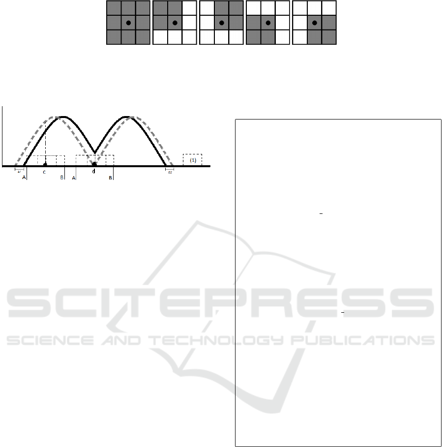
(a) (b) (c) (d) (e)
Figure 3: Illustration of shifting window around the examined point. (a): The classic KLT window where the point is always
at the center.(b), (c), (d), (e): different positions of windows are applied around the point, each of them leads to a different
motion value.
Figure 4: An 1-D illustration shows how the convergence
of estimated flows can be a criterion for reliability. We
suppose that the dotted gray line is a profile of intensity
from the previous image I
1
while the black line represents
the same profile I
2
after motion (∆
1
and ∆
2
are two dif-
ferent movement directions). The abscissa axis represents
the coordinates of the point and the ordinate axis represent
its intensity. For each point ”c”, ”d”, the window (1) will
slide in interval [A-B]. Intuitively, the window centered in
”c” would collect motion values of good uniformity with a
value close to ∆
1
. On the contrary, the flows collected in the
window centered in ”d” are scattered between ∆
1
and ∆
2
.
If
c
w
r
(p) ≥ w
r
(p)
u
e
(p) =
b
u
e
(p)
w
r
(p) =
c
w
r
(p)
(13)
Introducing the color similarity helps propagating
the flow in an object-oriented way in which the points
of close colors get more influence from each other
than the others.
5 IMPLEMENTATION
The numerical implementation of our method is given
in Table.1. The scheme of pyramidal images and
propagation of flows through pyramidal images are
implemented in the similar way as in (Wedel et al.,
2009). We focus here on the essential part of the pro-
posed method.
6 EXPERIMENTS
Our new algorithm is applied to the Middlebury
database in order to evaluate its performances for
small movements. The experiments are conducted by
Table 1: Implementation of the proposed algorithm.
Input: Two color images I
1
and I
2
Output: Flow vector u from I
1
to I
2
• Convert color images to gray I
1
→ G
1
, I
2
→ G
2
• Create L-levels pyramidal images for I
1
, I
2
,G
1
,
G
2
• Initialize u
L
= u
0
= 0
For l = L to 1
• Compute ∇I
l
1
(x), ∇G
l
1
(x)
For i = 1 to Max Warps
• Interpolate I
l
2
(x + u
l
), G
l
2
(x + u
l
)
• Compute ∇I
l
2
(x + u
l
),∇G
l
2
(x + u
l
)
• Compute I
l
t
• Compute {s ∈ S} and determine the weight
w
r
according to (7) by using G
1
,G
2
and their
derivations
• Estimated u
e
from S following (9)
• Modify u
l
by using w
r
and I
l
2
(x + u
l
):
For j=1 to Max Iteration
I Calculate
b
u
e
,
c
w
r
for all of the pixels
according to (11),(12)
I Collect the points whose
c
w
r
> w
r
I Modify their flow and reliable
score according to (13)
End
• Apply median filter to u
l
• Prepare the next iteration u
k−1
= u
l
End
• Propagate u
l
to u
l−1
• u
k
= u
l−1
End
using the pyramidal images and wrapping scheme to
well estimate the flow. To find the flow using the local
KLT method, we use a window size of 5× 5 applied to
the gray image. To propagate the flow using equation
(13), color is considered as explained in previous sec-
tions and neighbors belong to a window of size 5×5.
Moreover, σ
c
= 25 and σ
d
= 2.
Section 4.1 details the process used for estimat-
ing a consensual flow from a set of estimated flows
by using a weighted average value. As mentioned be-
fore, in order to test the robustness of the consensual
approach, three other possibilities have been tested:
using a random flow among the solutions, using the
closest solution from the constraint line and finally the
Optical Flow Refinement using Reliable Flow Propagation
455

Figure 5: Distribution of estimated flows for each point after shifting the estimation windows. We create a cloud of solution
S at each point.
original flow proposed in the KLT method. Table.2
and Table.3 show the error measures AAE
2
and EPE
3
after the propagation (Baker et al., 2010) for each ap-
proach and confirms the relevance of the weighted av-
erage.
Table 2: Accuracy of different strategies to choose a unique
flow from the set of candidates of two sequences Venus and
RubberWhale.
Database Venus RubberWhale
Approach AAE EPE AAE EPE
Average weight 4.054 0.261 3.558 0.114
Random 4.096 0.273 3.656 0.116
Closest 4.219 0.277 3.606 0.116
KLT 4.167 0.267 3.671 0.117
Table 3: Accuracy of different strategies to choose a unique
flow from the set of candidates of two sequences Grove2
and Urban2.
Database Grove2 Urban2
Approach AAE EPE AAE EPE
Average weight 2.514 0.170 3.919 0.518
Random 2.519 0.171 3.977 0.508
Closest 2.544 0.173 3.925 0.53
KLT 2.537 0.172 3.975 0.522
In order to show the relevance of our reliability
score, Fig.6 display respectively the real errors AAE
and EPE with respect to the reliability scores ranked
in decreasing order (the value 0 corresponds to the
highest reliability score), before and after propaga-
tion. First of all, the most reliable scores are actu-
ally related to a low error. Then, the propagation has
reduced the errors magnitude in a significant way.
Final error measures for the height images are col-
lected in Table.4. They are compared with the re-
sults provided by KLT (yves Bouguet, 2000), Horn
and Schunk with λ = 10 (Horn and Schunck, 1981),
Black and Anandan(BA) (Black and Anandan, 1996)
that has the same form of energy function with Horn
and Schunk but different error functions. In this case,
2
Average Angular Error
3
End Point Error
BA uses the robust function Geman-McLure. We use
the 8 sequences for which the ground truth is available
on the MiddleBury website
4
.
Experiments show that our method gives better re-
sults than the classic KLT or Horn and Schunck meth-
ods. Concerning the comparison with BA method,
our method has greater performance on real scenes
like (”RubberWhale”,”Hydrangea”,”Dimetrodon”).
However, when using synthetic images
(”Groove2”,”Groove3”,”Urban2”,”Urban3”), our
approach still could be improved to distinguish better
multiple flows that correspond to multiple motion in
small regions, as visible in Fig. 7(c). Because the
propagation is quite slow, with only 50 iterations,
the reliable score is difficult to reach at every pixel.
Hence, we can only correct the optical flow in a small
region around the reliable motion. In some images,
different false estimated motions in a large region
can cause consequently a false reliable flow to be
propagated as it is shown in Fig. 7(d) (the blue line).
We can note that some of the problems that were
mentioned before come from the inherent inaccuracy
of KLT as it uses only intensity to estimate flow.
7 CONCLUSION
Starting from a classical optical flow method like
KLT, we have proposed a new approach to improve
optical flow precision by exploiting a flow reliabil-
ity measure and a propagation strategy based on color
and proximity. The advantage of this new strategy
is to estimate the optical flow more precisely through
propagation of reliable flows. Note that the idea could
be extended to other optical flow techniques.
First results are promising as they show that our
approach give better results than two classic methods
(KLT and Horn and Schunk). The method is ranked
80/120 in the Middleburry evaluation
Moreover, our basic idea could be easily extended
by considering other image features such as texture
4
http://vision.middlebury.edu/flow/data/
VISAPP 2017 - International Conference on Computer Vision Theory and Applications
456
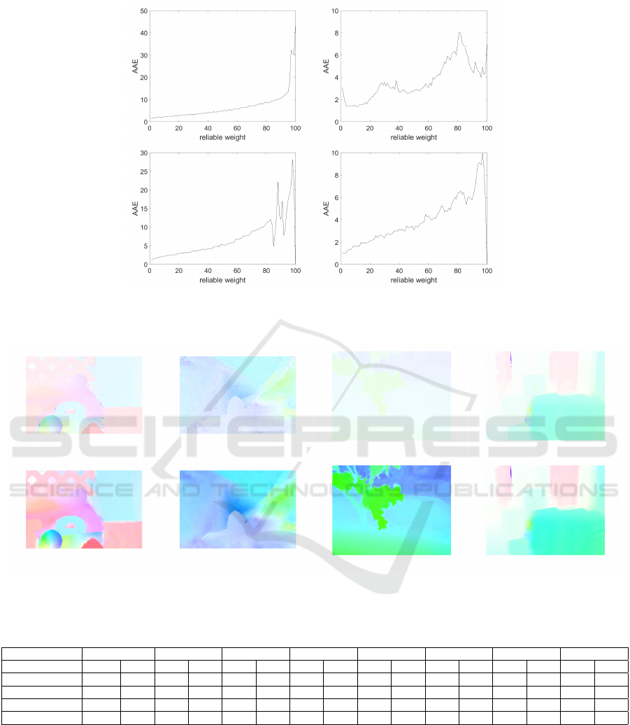
(a) (b)
Figure 6: Relation between reliable weight vs. AAE on two sequences (top: RubberWhale, bottom: Urban2): a) AAE before
propagation b) AAE after propagation.
(a) (b) (c) (d)
Figure 7: Optical flow before (first line) and after propagation (second line).
Table 4: Performance of the compared methods in the Middlebury database.
Database Venus Dimetrodon Hydrangea RubberWhale Groove2 Groove3 Urban2 Urban3
Method AAE EPE AAE EPE AAE EPE AAE EPE AAE EPE AAE EPE AAE EPE AAE EPE
Proposed method 4.054 0.261 3.877 0.194 2.422 0.221 3.558 0.114 2.514 0.170 5.940 0.624 3.919 0.518 4.429 0.739
KLT 10.737 0.729 5.958 0.289 3.756 0.328 6.113 0.203 3.143 0.231 7.21 1.043 7.262 1.035 7.989 2.194
HnS 5.6 0.34 4.767 0.232 3.008 0.257 5.175 0.16 2.719 0.196 6.315 0.649 4.924 0.562 6.943 0.756
BA 4.095 0.255 4.199 0.205 2.665 0.231 4.384 0.132 2.274 0.159 5.711 0.584 2.804 0.355 3.528 0.456
or gradient and then by considering other reliability
measures. Future work will consider other image fea-
tures and try to reduce computational cost.
REFERENCES
Bab-Hadiashar, A. and Suter, D. (1998). Robust Optic Flow
Computation. International Journal of Computer Vi-
sion, 29(1):59–77.
Baker, S., Scharstein, D., Lewis, J. P., Roth, S., Black, M. J.,
and Szeliski, R. (2010). A Database and Evaluation
Methodology for Optical Flow. International Journal
of Computer Vision, 92(1):1–31.
Black, M. J. and Anandan, P. (1991). Robust dynamic mo-
tion estimation over time. In , IEEE Computer Society
Conference on Computer Vision and Pattern Recogni-
tion, 1991. Proceedings CVPR ’91, pages 296–302.
Optical Flow Refinement using Reliable Flow Propagation
457

Black, M. J. and Anandan, P. (1996). The Robust Estima-
tion of Multiple Motions: Parametric and Piecewise-
Smooth Flow Fields. Computer Vision and Image Un-
derstanding, 63(1):75–104.
Brox, T. and Malik, J. (2011). Large Displacement Optical
Flow: Descriptor Matching in Variational Motion Es-
timation. IEEE Transactions on Pattern Analysis and
Machine Intelligence, 33(3):500–513.
Brox, T. and Weickert, J. (2002). Nonlinear Matrix Diffu-
sion for Optic Flow Estimation. In Gool, L. V., editor,
Pattern Recognition, number 2449 in Lecture Notes
in Computer Science, pages 446–453. Springer Berlin
Heidelberg. DOI: 10.1007/3-540-45783-6 54.
Chen, Z., Jin, H., Lin, Z., Cohen, S., and Wu, Y.
(2013). Large Displacement Optical Flow from Near-
est Neighbor Fields. pages 2443–2450. IEEE.
Farneback, G. (2000). Fast and accurate motion estimation
using orientation tensors and parametric motion mod-
els. volume 1, pages 135–139. IEEE Comput. Soc.
Horn, B. K. and Schunck, B. G. (1981). Determining optical
flow. Artificial Intelligence, 17(1-3):185–203.
Kim, T. H., Lee, H. S., and Lee, K. M. (2013). Optical Flow
via Locally Adaptive Fusion of Complementary Data
Costs. pages 3344–3351. IEEE.
Liu, H., Chellappa, R., and Rosenfeld, A. (2003). Accurate
dense optical flow estimation using adaptive structure
tensors and a parametric model. IEEE Transactions
on Image Processing, 12(10):1170–1180.
Lucas, B. D. and Kanade, T. (1981). An Iterative Image
Registration Technique with an Application to Stereo
Vision. pages 674–679.
Middendorf, M. and Nagel, H. H. (2001). Estimation and
interpretation of discontinuities in optical flow fields.
In Eighth IEEE International Conference on Com-
puter Vision, 2001. ICCV 2001. Proceedings, vol-
ume 1, pages 178–183 vol.1.
Nagel, H.-H. and Gehrke, A. (1998). Spatiotemporally
adaptive estimation and segmentation of OF-fields. In
Burkhardt, H. and Neumann, B., editors, Computer
Vision — ECCV’98, number 1407 in Lecture Notes
in Computer Science, pages 86–102. Springer Berlin
Heidelberg. DOI: 10.1007/BFb0054735.
Sun, D., Roth, S., and Black, M. J. (2010). Secrets of opti-
cal flow estimation and their principles. pages 2432–
2439. IEEE.
Wedel, A., Pock, T., Zach, C., Bischof, H., and Cremers,
D. (2009). An Improved Algorithm for TV-L 1 Op-
tical Flow. In Hutchison, D., Kanade, T., Kittler, J.,
Kleinberg, J. M., Mattern, F., Mitchell, J. C., Naor, M.,
Nierstrasz, O., Pandu Rangan, C., Steffen, B., Sudan,
M., Terzopoulos, D., Tygar, D., Vardi, M. Y., Weikum,
G., Cremers, D., Rosenhahn, B., Yuille, A. L., and
Schmidt, F. R., editors, Statistical and Geometrical
Approaches to Visual Motion Analysis, volume 5604,
pages 23–45. Springer Berlin Heidelberg, Berlin, Hei-
delberg.
Weinzaepfel, P., Revaud, J., Harchaoui, Z., and Schmid, C.
(2013). DeepFlow: Large displacement optical flow
with deep matching. In IEEE Intenational Conference
on Computer Vision (ICCV), Sydney, Australia.
Xu, L., Jia, J., and Matsushita, Y. (2010). Motion detail
preserving optical flow estimation. pages 1293–1300.
IEEE.
Yang, J. and Li, H. (2015). Dense, accurate optical flow
estimation with piecewise parametric model. pages
1019–1027. IEEE.
yves Bouguet, J. (2000). Pyramidal implementation of the
lucas kanade feature tracker. Intel Corporation, Mi-
croprocessor Research Labs.
VISAPP 2017 - International Conference on Computer Vision Theory and Applications
458
