
Explicit Image Quality Detection Rules for
Functional Safety in Computer Vision
Johann Thor Mogensen Ingibergsson
1,2
, Dirk Kraft
2
and Ulrik Pagh Schultz
2
1
CLAAS E-Systems, Møllevej 11, 2990 Niv
˚
a, Denmark
2
University of Southern Denmark, The Mærsk Mc-Kinney Møller Institute,
Campusvej 55, 5230 Odense M., Denmark
{jomo, kraft, ups}@mmmi.sdu.dk
Keywords:
Safety, Functional Safety, Image Quality Assessment, Low-level Vision.
Abstract:
Computer vision has applications in a wide range of areas from surveillance to safety-critical control of au-
tonomous robots. Despite the potentially critical nature of the applications and a continuous progress, the
focus on safety in relation to compliance with standards has been limited. As an example, field robots are
typically dependent on a reliable perception system to sense and react to a highly dynamic environment. The
perception system thus introduces significant complexity into the safety-critical path of the robotic system.
This complexity is often argued to increase safety by improving performance; however, the safety claims are
not supported by compliance with any standards. In this paper, we present rules that enable low-level detection
of quality problems in images and demonstrate their applicability on an agricultural image database. We hy-
pothesise that low-level and primitive image analysis driven by explicit rules facilitates complying with safety
standards, which improves the real-world applicability of existing proposed solutions. The rules are simple
independent image analysis operations focused on determining the quality and usability of an image.
1 INTRODUCTION
Safety certification of a robotic system concerns re-
liability towards errors identified in a manual safety
analysis. The computer vision domain however of-
ten neglects this issue because requirements often are
stated in terms of the performance of specific func-
tions, as stated by Yang et al. “one [issue] is to iden-
tify an obstacle surrounding the robot and the other
is to determine the location of the obstacle” (Yang
and Noguchi, 2012). This limited view could be the
result of the domain’s focus on developing and im-
proving solutions (Ingibergsson et al., 2015). There
is a focus on probabilistic measures for failure de-
tection based on analysis of distributions and using
learning methods (Blas and Blanke, 2011; Wang and
Bhanu, 2005; Zhang et al., 2014). The issue with
these methods is that it is difficult to prove that the
distributions cover the entire normal behaviour, as il-
lustrated by the spurious behaviour learning methods
can exhibit where images are indistinguishable for hu-
mans, but the neural network makes wrong classifica-
tions (Nguyen et al., 2015; Szegedy et al., 2013). A
key problem is that classifiers and learning are com-
plex tasks that are hard to prove reliable for humans,
in particular through code reviews, which is an often-
used procedure during safety certification.
Safety certification is a method for achieving
industry-required levels of reliability and dependabil-
ity, while addressing liability (for liability see (San-
tosuosso et al., 2012)). Compliance with safety
standards is considered key to ensuring reliabil-
ity by achieving an appropriate level of functional
safety (TC 23, 2015). Critically, complying with
safety standards is not about the systems nominal per-
formance, functional safety should rather be viewed
as guaranteed reliability towards specific errors with
regards to the entire system (hardware components,
hardware design and software) or as guaranteed re-
action, e.g. reaching a safe state. Functional safety
is a matter of firstly conducting a Hazard and Risk
Analysis (HRA), where hazards are errors or failures
of functions that the system relies upon called safety-
related functions. A safety-related function could be
detecting humans, where a hazard is that the image is
overexposed, resulting in missed detections. The risk
analysis of the hazards imposes requirements on the
entire development process, through the formulation
of safety goals. A safety goal would be to ensure that
the image exposure is usable for the algorithms. Each
Ingibergsson J., Kraft D. and Pagh Schultz U.
Explicit Image Quality Detection Rules for Functional Safety in Computer Vision.
DOI: 10.5220/0006125604330444
In Proceedings of the 12th International Joint Conference on Computer Vision, Imaging and Computer Graphics Theory and Applications (VISIGRAPP 2017), pages 433-444
ISBN: 978-989-758-227-1
Copyright
c
2017 by SCITEPRESS – Science and Technology Publications, Lda. All rights reserved
433

safety goal will result in the development of safety
function(s), that ensure or monitor that the safety goal
will not be violated (Zenke et al., 2016). The safety
functions need to be human-understandable to reflect
the connection between the safety goals and the haz-
ards, as to enable the certification authorities to certify
the system based on code review. A safety function
could, therefore, be to evaluate the fill level of bins
in a histogram. We observe that safety certification is
especially important for vision pipelines used for the
autonomous operation of robots and vehicles operat-
ing in dynamic environments since the vision pipeline
introduces an increased risk of failures in critical parts
of the robots’ functionality. Indeed, outdoor mobile
robots fail up to ten times more often than other types
of robots (Bansal et al., 2014; Carlson et al., 2004).
This paper uses field robots operating on an agricul-
tural field as sample domain.
We hypothesise that the use of explicitly written
easily understandable computer vision rules supports
certification authorities in reviews, and thereby pro-
vides an increased understanding of the system safety
functions and functionality. The safety-critical func-
tions are limited to simple tests on the images to ver-
ify the quality and functionality of the camera system.
We hypothesise that these functions can ensure that
the data stream is of high quality and that the images
are reliable, thus verifying that a higher-level vision
algorithm is given the pre-required quality to perform
optimally, making the system as a whole more reli-
able. In this paper, we test different rules to ascer-
tain the usability and applicability of a proposed set
of simple rules, and we have conducted experiments
that demonstrate the viability of the proposed rules.
The paper is structured as follows. In Section
2 we describe standards applicable for certification
of vision systems and relevant sub-domains such as
learning and hazards analysis. Section 3 introduces
our proposed method of using simple explicit writ-
ten imaging rules, along with methods, new concepts
and dataset used in this paper. Section 4 is the ini-
tial verification of the rules tested using the area un-
der the precision recall curves. Section 5 introduces
an augmentation to the rules called soft-boundaries,
were we experiment with multi-classifications to im-
prove applicability for safety certification. In Section
6 we randomly split the dataset to verify the results
and that the dataset is sufficient for preliminary con-
clusions. In Section 7 we have an overall discussion
of the results and the validity of the study, ending with
Section 8 with an overall conclusion for the work.
2 BACKGROUND AND RELATED
WORK
This section first discusses functional safety in the
context of computer vision, then gives an overview of
current research in computer vision relevant to func-
tional safety, and last reviews learning methods in the
context of functional safety.
2.1 Safety Certifying Vision Systems
Functional safety standards only address human dan-
gers, e.g., within agriculture ISO 25119 (TC 23,
2010). This leaves the designer and developer to cate-
gorise issues related to harming the robot, e.g. hitting
non-human obstacles. This means that safety should
be addressed for the entire operation of the robot, em-
phasising the need for compliance and certification.
No specific standards however cover the do-
main of robotic vision systems or outdoor robotics.
Mikta et al. (Mitka et al., 2012) introduced an ini-
tial idea using national standards. Some of these
concepts have been introduced in newer standards
for robots, such as ISO 13482 (TC 184, 2014).Func-
tional safety standards such as ISO 25119 for agricul-
ture (TC 23, 2010), and ISO 13482, for personal care
robots (TC 184, 2014), are important for the overall
functional safety of the robot, and also for the sub-
systems. Specific for vision systems a standard exist
for vision in industrial setting, IEC 61496 (TC 44,
2012) which could be usable, as would upcoming
standards for performance of vision systems (TC 23,
2014; TC 127, 2015). These standards cover the de-
sign of hardware as well as software, which makes it
cumbersome to get complex systems and algorithms
certified.
The functional safety standards introduce the con-
cept of safe states which are important during faults
or malfunctions. Sensors, in general, have a risk of
failing, where common sensor faults are sensor bias,
locked in place and loss of calibration (Daigle et al.,
2007). These failures are malfunctions which re-
quire that the sensors are robust, without robustness
the robot may “hallucinate” and respond inappropri-
ately (Murphy and Hershberger, 1999). It is there-
fore important for functional safety to look at software
safety verification of the input image, and thereby to
give assurance about the hardware and verifying in-
puts and outputs.
The importance of computer vision being com-
pliant and certified is due to its use in connection
with real-time control of autonomous systems, such
as vehicles (Cheng, 2011) and robots (De Cabrol
et al., 2008). For this reason, verifiability of con-
VISAPP 2017 - International Conference on Computer Vision Theory and Applications
434

trollers is important (Bensalem et al., 2010). Barry et
al. propose a safety-verified obstacle avoidance algo-
rithm (Barry et al., 2012) to enable Unmanned Aerial
Vehicles (UAVs) to sense and avoid obstacles. How-
ever, the underlying data the system receives is not
evaluated, and therefore implicitly requires trustwor-
thy data and images. Despite the missing standards
there have been steps towards verifying computer vi-
sion test data (Zendel et al., 2015; Torralba and Efros,
2011). Zendel et al. investigate test data using Hazard
and Operability Analysis (HAZOP). which is a sys-
tematic examination of a process (e.g. computer vi-
sion) used to identify problems that represent a risk to
personnel or equipment. As a complementary effort,
we aim to identify safety functions that can be used
to ensure that the system is able to detect failures and
return to a safe state.
We hypothesise that the use of explicitly written
computer vision rules supports certification authori-
ties in reviews, providing an increased understanding
of the systems safety functions and the functionality;
similar approaches with simple rules to facilitate cer-
tification exists for other domains (Adam et al., 2016).
2.2 Learning Methods
Safety certification of neural networks (Kurd and
Kelly, 2003) remains an open issue. Specifically,
Kurd et al. refer to Artificial Neural Networks (ANN)
that are understandable and readable by humans, and
also allows for individual meaningful rules (Kurd and
Kelly, 2003). Many industries have looked into the
use of ANN (Schumann et al., 2010). Specifically, in-
dustries not related to agriculture, like aerospace and
military. These industries have been investigating the
use of ANN since the 1980s (Schumann et al., 2010).
A particular interesting approach is from Gupta et
al. looking into verification and validation of adap-
tive ANN (Gupta et al., 2004), although Gupta et al.
focus on control systems. These ideas are mainely
aimed at ensuring that the ANN will not react un-
controllably based on bad images, and that outputs
can be controlled. However, there does not exist a
standard to comply with for ANN systems, specifi-
cally the absence of analytical certification methods
restricts ANN to advisory roles in safety-related sys-
tems (Kurd et al., 2003). We hypothesise the use of
low-level safety as a means to be compliant with stan-
dards and thereby enable the use of high-level more
complex vision systems for performance. Moreover,
we note that deep neural networks and similar re-
cently popular methods share the same issue of being
hard to assess.
Zhang et al. describe the before mentioned sys-
tems as BASESYS (Zhang et al., 2014). They ar-
gue that introducing an evaluation would enable the
BASESYS to have a measure of whether or not at-
tributes are reliable for later detection schemes. A
method proposed by Bansal et al. (Bansal et al., 2014)
suggests to create a classifier that predetermines the
“quality” of an image, but the authors argue that this
boosts performance. Performance is a criterion that is
highly sought for in the computer vision domain, e.g.
for pedestrian detection (Doll
´
ar et al., 2010). How-
ever, functional safety does not deal with nominal per-
formance of the system. Our approach would be to
use low-level image analysis instead of high-level at-
tributes as Zhang et al. do..We believe this facilitates
compliance with safety standards, and generally im-
proves the reliability of systems dependent on vision.
3 EXPLICIT IMAGE QUALITY
DETECTION
We now introduce the concept of explicitly written
computer vision rules, which is the basis of this pa-
per. These rules will be initially analysed in Sec-
tion 4. This analysis is based on Precision-Recall
(PR) curves which are introduced after the rules. We
want to enable certification and use of many sensors
on a robotic system; we, therefore, introduce a con-
cept called multiclass classification, as seen in other
safety critical systems (Mekki-Mokhtar et al., 2012).
In this preliminary study, we will focus on only three
classes “bad”, “warning” and “good”. This will en-
able the decision system to decide the trustworthiness
of different sensors, and thereby decide if the robot
needs to stop or just slow down. Finally, because of
the introduction of multiclass classification, we intro-
duce a concept we call soft boundaries into our eval-
uation strategy, to ensure that small misclassifications
are not penalised.
3.1 Rules
We choose explicit image quality detection rules that
are computationally simple, and contribute to the test
of our hypothesis, as follows;
1. Filled Bins Ratio of a Histogram (FB): The FB
rule is based on histogram analysis. The analysis
is the relation between the number of bins with
pixels divided by the total number of bins. For
a bin to be categorised as having pixels it has to
have more than 100px to remove noise. Example
hazard: Exposure.
Explicit Image Quality Detection Rules for Functional Safety in Computer Vision
435

FB =
non empty bins
total bins
=
number o f (bin)
∑
i=1
(#bin
i
>100px)
number o f (bin)
2. Bin Distribution, Maximum vs. Minimum Bin
(BN): This rule finds the bin with most pixels and
subtracts the pixel value with the pixel value of
the bin with the lowest amount of pixels. The re-
sult is then divided by the total amount of pixels.
Example hazard: Covered image.
BN =
Max(#bin
i
)−Min(#bin
j
)
total pixels
=
Max(#bin
i
)−Min(#bin
j
)
img width·img height
, #bin
i, j
> 100
3. Bin Fill Ratio in a Histogram Uniform (BF):
This rule is an extension to the BN rule, where
this is the difference between the individual bins
and the total amount of pixels. Example hazard:
Exposure.
BF =
Max(#bin
i
)
total pixels
=
Max(#bin
i
)
img width·img height
4. Energy Ratio Before and After High-pass Fil-
tering (FR): The image is filtered using a very
aggressive high-pass filter (second order Butter-
worth filter applied in the frequency domain with
a cutoff frequency of the full image). The rule
then compares the energy of the image after fil-
tering and before (representative of the relatively
high-frequency energy content in the image). This
gives a notion about the high-frequency content /
sharpness of the image. Example hazard: Blurred
image.
FR =
energy a f ter f ilter
total energy
=
BW f ilter(img)
total energy(img)
5. Component Analysis (CA Top & Bottom):
Connected component analysis is used for finding
over (e.g. sunshine) and under (e.g. covered im-
age) exposed spots on the image. The rule works
on binary images; therefore thresholding is used
with thresholds of < 10 for the bottom, and > 245
for the top. After which, connected components is
used, and the area of the biggest component is out-
put. The rule is able to catch significant light and
dark spots on the image. Example hazard: Over-
exposed image.
CA = {max(area(component
i
)) : component
i
∈
image}
6. Optical Flow (OF): Optical flow using Lucas
Kanade (Lucas et al., 1981) uncovers if an im-
age is changing. This is done by evaluating how
many areas of the image are moving above a cer-
tain threshold. Example hazard: Stuck image.
OF =
∑
(movement(area
i
)>0.2)
total areas
=
number o f (area)
∑
i=1
(movement(area
i
)>0.2)
number o f (area)
All of the rules above use a threshold that defines if
the image violates the rules. In this paper, we seek
to define optimum thresholds for the individual rules.
The rules were initially assessed individually to un-
derstand their applicability to distinguish “bad” from
“good” images. This analysis is done in Section 4,
where we have evaluated the individual rules on their
own, by assessing their statistical attributes by look-
ing at the Precision-Recall (PR) curves.
3.2 Precision-Recall
We used PR curves to identify the performance of
the classifiers without having to choose a particular
threshold. PR curves are chosen over Receiver Oper-
ating Characteristics (ROC), because we know that if
a curve dominates in the PR-space, it will also dom-
inate in the ROC space (Davis and Goadrich, 2006).
Furthermore, ROC does not take the baseline into ac-
count, and since our categories are unbalanced, the
PR-curves are a better statistical measure. Because
we use PR for evaluation, we will use a trapezoidal
approximation of the Area Under the Curve (AUC)
to evaluate the resulting PR curves, to find an “op-
timum”, this is because linear approximation is in-
sufficient for PR (Davis and Goadrich, 2006). The
use of AUC on PR instead of ROC is further sup-
ported by Saito et al. “The PRC [Precision-ReCall]
plot is more informative than ROC, CROC [Concen-
trated ROC], and CC [Cost Curve] plots when evalu-
ating binary classifiers on imbalanced datasets” (Saito
and Rehmsmeier, 2015). With the hope of using these
methods in connection with functional safety, a per-
fect score would be desirable, however not a plausi-
ble result to aim for. The results will, therefore, be
used to decide upon which rules are feasible to test
with the following multiclass classification and soft
boundaries schemas.
3.3 Multiclass Classifications
In addition to the initial analysis of using PR, we want
to extend the investigations, by not only assessing the
image as “good” or “bad”, as normally done when
using PR. Instead, we want to introduce another re-
gion to improve the initial results. This we want to do
by introducing a two-step classification and thereby
an additional classification region, which is a system
“warning”. The concept of a warning region within
safety systems for autonomous robots has also been
introduced by Mekki-Mokhtar et al. (Mekki-Mokhtar
et al., 2012). This would make the system able to cat-
egorise three regions “error”, corresponding to “bad”,
“warning”, and “good”. The flow is illustrated in Fig-
VISAPP 2017 - International Conference on Computer Vision Theory and Applications
436
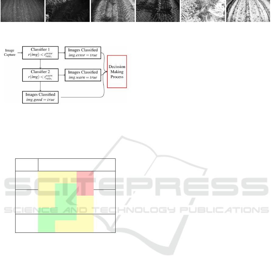
Figure 1: Exemplary images of field recordings done by a major agricultural company. The images are of crop structures and
the ground, taken with a front facing camera placed on an agricultural machine.
Figure 2: Concept of the extended classification approach,
showing how the image propagates and how the system is
told / made aware of the different steps. t is the threshold
where ∀t, i : t
error
rule
i
6= t
warn
rule
i
, and r is the rule, finally img
stands for the current image.
Table 1: Example of the soft boundary region, enabling an
overall system evaluation using PR curves.
Region
Covered Good Warning Error Zone
1 FP FP TN Error
2 FP FP TN Region
3 FP TP TN
4 FP TP TN
5 FP TP FN Warning
6 FP TP FN Region
7 TP TP FN
8 TP TP FN
9 TP FN FN Good
10 TP FN FN Region
ure 2. Mokhtar et al. state that “The set of warning
states represents the safety margin between nominal
safe states and catastrophic states, i.e. those corre-
sponding to hazardous situations” (Mekki-Mokhtar
et al., 2012), inferring that more classes are possible
to implement. The split into different regions would
facilitate later combination of the rules, i.e. if a certain
combination of rules produces warnings then the sys-
tem could also interpret this as an error, we, however,
leave this to future work.
3.4 Soft Boundaries
Soft boundary refers to the classification region for
each of the rules. We want to make the transition
smooth by allowing “small misclassifications”. This
is accomplished by moving the False Positive (FP)
and False Negative (FN) that are calculated for the
given PR curve, into the respective blocks True Posi-
tive (TP) or True Negative (TN), of course, this is only
done within the soft boundary region. To exemplify
both the soft boundaries and the “bad”, “warning” and
“good” regions, we choose the category covered and
give the example in Table 1.
For this example the ground truth is specified such
that all images below four (1-3) are “bad” and above 7
are good (8-10), then the warning region is in between
(4-7). Where it normally is a strict line we propose a
boundary region, example ±1. When the analysis for
the PR is made, the boundary region influences the
FN and FP, in the following way:
• If an image hand labelled as 3 is categorised as
“Warning”, it is a FP. But because of our boundary
region, this would not be an error; the data should,
therefore, be interpreted as a TP.
• In the reverse example if an image hand labelled
as 4 is categorised as “bad” corresponding to FN,
it should be accepted and therefore be interpreted
as a TN.
These two regions and the soft boundary concept
is introduced as not to penalise the system for misclas-
sifying some images as “warnings” or “errors”. This
should of course only be done in the soft boundary
region, because classifying an image that is “good”
or close to “good” as an error should still be an is-
sue. This follows the idea from our hypothesis that
our rules evaluate the images as shown in Figure 2.
This enables the decision system to act based on the
trustworthiness and functional safety of the system.
Thereby making the system able to react by lowering
speeds and/or relying more on other sensors to keep
the system trustworthy.
3.5 Dataset
This paper focuses on images similar to those shown
in Figure 1. The images come in pairs since they are
recorded with a stereo camera. To enable the evalua-
tion of the method 406 random images from the large
database have been manually evaluated based on five
criteria exposure, movement, sharpness, covered and
usable. These are evaluated based on the different cri-
teria listed in Table 2, resulting in the classification of
406 sample images shown in Table 3. The images
have a resolution of 752x480 or 1280x1024.
Explicit Image Quality Detection Rules for Functional Safety in Computer Vision
437
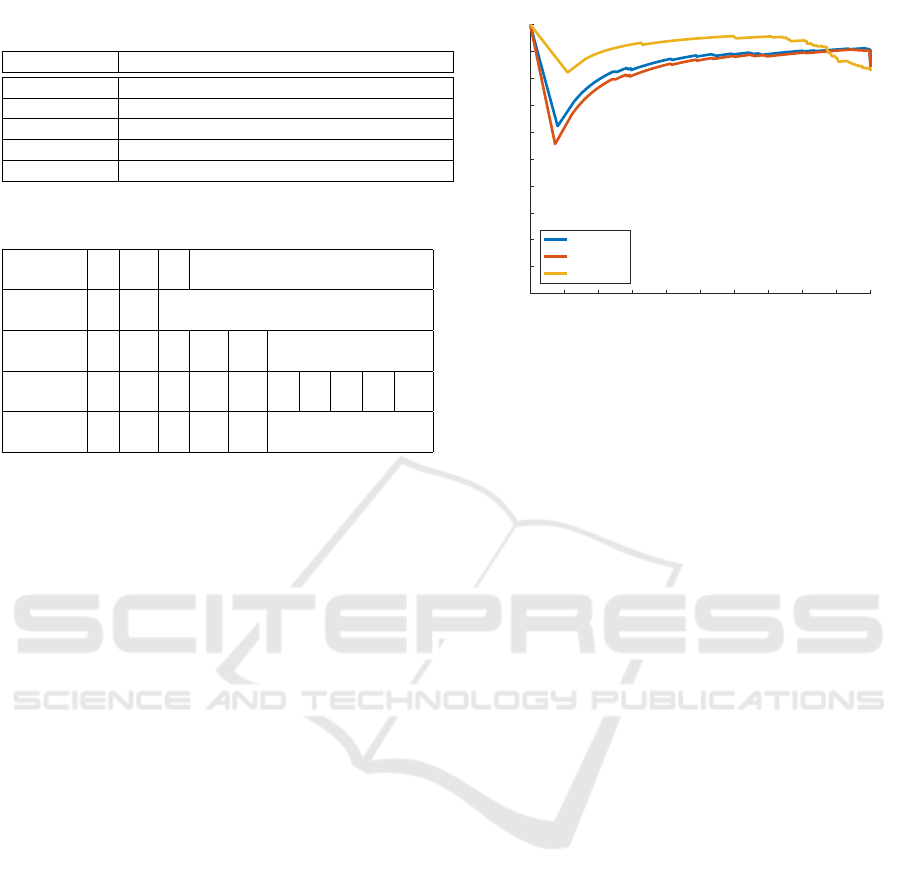
Table 2: Overview of the classification criteria for the five
image categories.
Category Description
Exposure (1-3) 1: Under exposure. 2: Okay. 3: Over exposure.
Movement (1-2) 1: No. 2: Yes.
Sharpness (1-5) 1: No structure. 2: 25%. 3: 50%. 4: 75%. 5: Perfect.
Covered (1-10) 1: Everything. 2-9: Percentage increase. 10: Nothing.
Usable (1-5) 1: Not usable. 2: Bad. 3: Average. 4: Good. 5: Perfect.
Table 3: Overview of the ground truth data classification of
the 406 sample images.
Exposure 1 2 3
(count) 70 288 48
Movement 1 2
(count) 86 320
Sharpness 1 2 3 4 5
(count) 28 30 49 156 143
Covered 1 2 3 4 5 6 7 8 9 10
(count) 1 1 6 7 16 38 30 33 35 239
Usability 1 2 3 4 5
(count) 36 30 57 114 169
4 SINGLE THRESHOLD
PERFORMANCE EXPERIMENT
In this section, we describe our approach and results
on using the rules presented in Section 3.1 individu-
ally, by assessing their statistical attributes by look-
ing at the resulting PR curves. Instead of creating a
learning scheme, we hypothesise that the creation of
distinct rules will facilitate certification of CV sys-
tems. As an example for what we will analyse we
choose the Fourier rule (FR). Using FR, we will try to
detect sharpness, covered and usable for understand-
ing what is possible to detect. The initial plots shown
in Figure 3, are where only the lowest score one
(for sharpness, covered and useable) is categorised as
“bad”, all others categories are “good” (please see Ta-
ble 2 for classification criteria and scores).
To enable and simplify an analysis we use AUC.
We are aware that the approximation can be incorrect
as per Davis et al. (Davis and Goadrich, 2006). We are
therefore manually inspecting the value during calcu-
lation to ensure that the trapezoidal approximation of
the AUC is plausible. This analysis of the particu-
lar case shown in Figure 3 results in the AUC shown
in Table 6, from the data we can conclude, per vi-
sual inspection on Figure 3 that the attribute covered
is the best attribute to be found using FR. However, it
should be noted that this is done using the classifica-
tion that the lowest value, i.e. one, means “bad” im-
age and the others are categorised as “good” values.
Based on Tables 2 and 3 categorising only a score of
one as “bad” might not be the most optimal. Addition-
0 0.1 0.2 0.3 0.4 0.5 0.6 0.7 0.8 0.9 1
0
0.1
0.2
0.3
0.4
0.5
0.6
0.7
0.8
0.9
1
sharpness - PR
sharpness
usable
Covered
Figure 3: Initial PR curve of the ability to use rule FR
for detecting “bad” images within the following categories:
Sharpness, covered and usable.
ally, it would be assumed that the correlation between
the sharpness and frequency would be much stronger
than shown in Table 6. For the analysis of all the
rules, we change the classification border for the PR
curves to find the optimal regions for distinguishing
between “good” and “bad” images. The best region
refers to finding the best classification of the ground
truth. This analysis is based on the found AUC for PR
curves and shown in Table 4. Comparing the results
in Table 4 with the results in Table 3, it is evident that
the first four categories for Covered are not that useful
because they only amount to 15 images out of the 406
images.
From Table 4 it can be seen that certain rules can
be used to detect certain attributes well. Because we
are looking at this in connection with certification, we
are interested in achieving as high PR scores as pos-
sible. In addition a classification of a “bad” image as
“good” could have catastrophic consequences in our
case. We have therefore tried to improve the results
by introducing multiclass categorization.
5 SOFT-BOUNDARY REGION
EXPERIMENT
In this section we describe our experiment of using
a multiclass approach in connection with soft bound-
aries to assess images.
5.1 Experiment
Defining the scope of the boundary analysis is done
based on the rules that are most promising within each
attribute, this evaluation is done based on the results
in Section 4:
VISAPP 2017 - International Conference on Computer Vision Theory and Applications
438
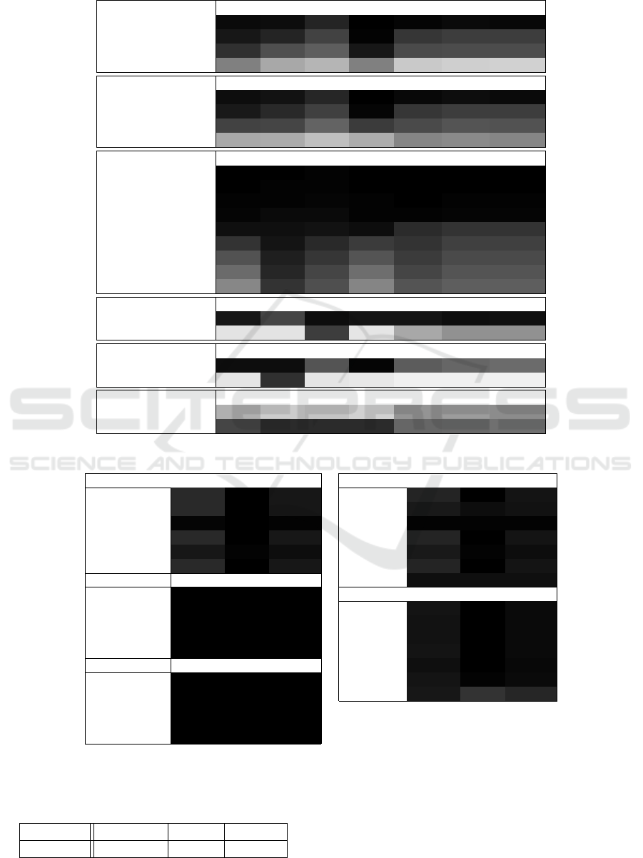
Table 4: Evaluating PR curves using AUC on all categorisations through the entire range. The colour scheme emphasises the
most relevant rules.
Sharpness FB BU BFU FR CA bot CA top OF
1:bad | 2-5 good 0.9618 0.9509 0.8621 0.9986 0.9789 0.9603 0.9658 [t]
1-2:bad | 3-5 good 0.9125 0.8554 0.7381 0.9875 0.7922 0.7649 0.7623
1-3:bad | 4-5 good 0.8136 0.6941 0.6276 0.9066 0.7146 0.7041 0.7024
1-4:bad | 5 good 0.4988 0.3421 0.2869 0.5001 0.2110 0.1890 0.1761
Usable FB BU BFU FR CA bot CA top OF
1:bad | 2-5 good 0.953 0.926 0.849 0.998 0.970 0.953 0.960
1-2:bad | 3-5 good 0.904 0.837 0.748 0.983 0.790 0.756 0.755
1-3:bad | 4-5 good 0.744 0.730 0.608 0.770 0.709 0.669 0.677
1-4:bad | 5 good 0.339 0.326 0.249 0.320 0.484 0.457 0.481
Covered FB BU BFU FR CA bot CA top OF
1:bad | 2-10 good 1.000 1.000 0.994 1.000 1.000 0.999 0.999
1-2:bad | 3-10 good 0.998 0.993 0.994 1.000 0.998 0.997 0.998
1-3:bad | 4-10 good 0.990 0.985 0.979 0.994 0.996 0.989 0.990
1-4:bad | 5-10 good 0.976 0.958 0.963 0.992 0.989 0.979 0.982
1-5:bad | 6-10 good 0.936 0.938 0.927 0.946 0.834 0.804 0.795
1-6:bad | 7-10 good 0.804 0.919 0.844 0.768 0.800 0.751 0.749
1-7:bad | 8-10 rest good 0.677 0.882 0.792 0.670 0.769 0.710 0.712
1-8:bad | 9-10 rest good 0.582 0.848 0.734 0.565 0.725 0.666 0.672
1-9:bad | 10 rest good 0.473 0.796 0.691 0.481 0.674 0.625 0.629
Over exposure FB BU BFU FR CA bot CA top OF
3:bad | 1-2 good 0.914 0.734 0.950 0.921 0.917 0.947 0.941
2-3:bad | 1 good 0.106 0.106 0.757 0.095 0.338 0.431 0.431
Under exposure FB BU BFU FR CA bot CA top OF
1:bad | 2-3 good 0.945 0.952 0.670 0.981 0.635 0.596 0.581
1-2:bad | 3 good 0.100 0.811 0.104 0.088 0.059 0.063 0.059
Movement FB BU BFU FR CA bot CA top OF
1-good | 2-bad 0.309 0.202 0.225 0.179 0.417 0.386 0.448
2-good | 1-bad 0.730 0.832 0.827 0.830 0.601 0.585 0.561
Table 5: Overview of the best F
1
scores and their accompanying precision-recall combinations, for the chosen rules.
Usable precision recall F1-score Sharpness precision recall F1-score
Rule FB 0.8374 1.0000 0.9115 Rule FB 0.8571 1.0000 0.9231
Rule BN 0.8374 1.0000 0.9115 Rule BN 0.9021 0.9511 0.9259
Rule BF 0.9828 1.0000 0.9913 Rule BF 0.9901 0.9925 0.9913
Rule FR 0.8374 1.0000 0.9115 Rule FR 0.8571 1.0000 0.9231
Rule CA bot 0.9052 0.9891 0.9453 Rule CA bot 0.9010 0.9945 0.9455
Rule CA top 0.8370 0.9971 0.9101 Rule CA top 0.8568 0.9971 0.9216
Under exposure precision recall F1-score Rule OF 0.9398 0.9398 0.9398
Rule FB 1.0000 1.0000 1.0000 Covered precision recall F1-score
Rule BN 1.0000 1.0000 1.0000 Rule FB 0.9236 1.0000 0.9603
Rule BF 1.0000 1.0000 1.0000 Rule BN 0.9261 1.0000 0.9616
Rule FR 1.0000 1.0000 1.0000 Rule BF 0.9282 1.0000 0.9628
Rule CA bot 1.0000 1.0000 1.0000 Rule FR 0.9236 1.0000 0.9603
Over exposure precision recall F1-score Rule CA bot 0.9378 0.9974 0.9667
Rule FB 1.0000 1.0000 1.0000 Rule CA top 0.9233 0.9947 0.9576
Rule BF 1.0000 1.0000 1.0000 Rule OF 0.9091 0.7979 0.8499
Rule FR 1.0000 1.0000 1.0000
Rule CA top 1.0000 1.0000 1.0000
Rule OF 1.0000 0.9951 0.9975
Table 6: The AUC value from the plot in Figure 3 approx-
imated, analysed according to the three categories chosen,
Sharpness, covered and usable.
sharpness usable covered
PR AUC 0.8554 0.8368 0.9186
1. Sharpness: Rule FB, Rule BN, Rule BF, Rule
CA (top and bottom) and Rule OF are the most
promising.
2. Usable: Rule FB, Rule BN, Rule BF, Rule FR and
Rule CA (top and bottom).
Explicit Image Quality Detection Rules for Functional Safety in Computer Vision
439

0 0.2 0.4 0.6 0.8 1
R
0
0.2
0.4
0.6
0.8
1
P
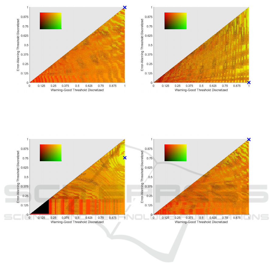
Figure 4: 2D plot of the precision-recall are made using BF
(Rule 3) and the sharpness measure. In addition, the blue
cross is the location of the highest F1 score. The colour
map in the corner depicts the relation between precision and
recall. The darkest yellow colour displays the highest sum
of the precision-recall measures, and grey is no data.
3. Covered: Rule FB, Rule BN, Rule BF, Rule FR,
Rule CA (top and bottom) and Rule OF.
4. Over Exposure: Rule FB, Rule BF, Rule FR,
Rule CA (top) and Rule OF. The border is FB bad,
BN warning and BF good.
5. Under Exposure: Rule FB, Rule BN, Rule BF,
Rule FR and Rule CA (bottom).
6. Movement: Not applicable because it is only di-
vided into two categories.
With the rules chosen for the investigation, the
thresholds need to be found, by changing the thresh-
old in steps between the minimum and maximum for
the specific dataset, different PR values are found.
However, since two thresholds are changed at the
same time, it is no longer valid to use AUC as above.
Instead, we use a colour map to show the individual
PR calculations for the changes in thresholds, because
we now have a precision and a recall value for each
point in the plot. The definition for the colour map is:
RGB(Red, Green, Blue) = RGB(Precision, Recall, 0)
In addition, an optimum point is chosen based on the
F
β
score. The F
β
score is a statistical measure that
can be used to evaluate the classification performance.
The β is a number reflecting a weight on either recall
or precision. We have chosen 1 which results in the
harmonic mean of precision and recall. The F
1
score
is a weighted average where the best value is at 1 and
the worst is 0.
An example plot for the analysis is shown in Fig-
ure 4. The chosen example is using the sharpness
measure and BF (Rule 3), which is divided into five
categories according to Table 2. The error→warning
Table 7: The result of combining the “error→warning” and
“warning→good” threshold, including the soft boundaries,
for Rule 4 “under exposure”.
Collected TP FP TN FN
1 70 0 0 0
2 288 0 0 0
3 48 0 0 0
threshold on the categories is set so that 1-2 is
categorised as “bad” and 3 is a “warning”. The
“warning→good” threshold is set at 4, meaning that
images in category 5 are categorised as “good”. The
images that have been categorised as “bad” could be
removed, but are not at this time.
The results in Figure 4 are found by changing the
two thresholds on the value of the outcome of the rule
in use (here BF - Rule 3), one for “bad→warning” and
one for “warning→good”. The use of the soft bound-
ary results in the precision-recall and the F1 score is
depicted on the Figure 4 as the blue cross. Concretely,
an F1-score of 0.9913 was found at the blue cross
in Figure 4, this is found using the combination of
precision 0.9901 and recall 0.9925. The specific val-
ues were found using the combination of thresholds
t
bad→warn
= 0.5106 and t
warn→good
= 0.1076, mean-
ing that if the most filled bin has more than half of all
pixels in it, the outcome is “error” and if it has less
than 10.76%, the outcome is “good”.
These results indicate that it is possible to create
simple rules relevant to this problem domain. The
same procedure is applied to all the relevant rules, re-
sulting in multiple F1 scores with their accompanying
precision-recall combinations, shown in Table 5.
5.2 Discussion of Results
Some results in Table 5 stand out as being very poor
or nearly too good to be true. As an example, “under
exposure” (Rule FR), seems to overperform strongly
compared to the initial results from Section 4 (see also
Figure 5a), and “sharpness” (Rule FR) seems to un-
derperform. The issue with “under exposure” is that
the category is only divided up into three subcate-
gories. This means that the soft boundary rule re-
moves FP and FN completely, an example can be seen
in Table 7, which imposes that ground truth categories
should be divided into more than three categories.
This means that we can only assess the categories
“usable”, “sharpness” and “covered”. Looking to the
other example chosen using “sharpness” on Figure 5b,
it shows that the optimal point is in the top right cor-
ner, suggesting that the manually labelled categories
are not precise enough or that the filter used is too
strong because this measure should be a strong indi-
cation of sharpness. Looking at the area where the
VISAPP 2017 - International Conference on Computer Vision Theory and Applications
440
0 0.2 0.4 0.6 0.8 1
R
0
0.2
0.4
0.6
0.8
1
P
(a) The result of using Rule FR as a means to determine
“under exposure”.
0 0.2 0.4 0.6 0.8 1
R
0
0.2
0.4
0.6
0.8
1
P
(b) The result of using Rule FR as a means to determine
“sharpness”.
Figure 5: Rule FR has been chosen, and two exemplary categories for under and over performance respectively. The blue
cross specifies the Highest F1 score.
0 0.2 0.4 0.6 0.8 1
R
0
0.2
0.4
0.6
0.8
1
P
(a) The result of using CA bot to determine “usability”.
0 0.2 0.4 0.6 0.8 1
R
0
0.2
0.4
0.6
0.8
1
P
(b) The result of using FR to determine “usability”.
Figure 6: “usability” is estimated to be the best-performing categorisation, plots illustrate the performance of example rules.
F1 score is the highest it is when “error→warning” is
close to maximum and “warning→good” is at maxi-
mum, resulting in an F1 score of 0.9231. Seeing that
the precision value is not that high, it might be pos-
sible to amend with a better filter. The results show
promise but emphasise the need for a bigger dataset.
The results in Table 5 indicate that further work
is interesting, especially when looking at the “usable”
category. Nearly all of the rules perform adequately,
despite some of them being at the extreme ends of the
plots (right edge), see Figure 6. On Figure 6a it can
be seen that the yellow region is a large area towards
the top (the blue cross could be multiple places, with
only small deterioration in F1-score), inferring that
this is a measure for detecting “usability”. Neverthe-
less, more data is needed to determine the effective-
ness of the rule. For Figure 6b, the F1 score is also
at its maximum one, see Table 5. Nevertheless, since
the optimal point is in the top right corner, it indicates
that the dataset is skewed, a larger dataset is therefore
needed to test the chosen threshold.
6 RANDOMISED VERIFICATION
TEST
As a preliminary verification of the found F1 scores
and their thresholds, we test our apporach by ran-
domly choosing half the labelled image dataset for
testing, corresponding to 203 images. The se-
lected images are used to find the optimal F1 score
and extract the “error→warning” threshold and the
“warning→good” threshold, as was done in Section 5.
The determined thresholds are then used on the re-
maining 203 images not used for defining the thresh-
olds. This is done to verify the detection capabilities
Explicit Image Quality Detection Rules for Functional Safety in Computer Vision
441

and the performance of the specific thresholds.
The test has been conducted for 200 runs, result-
ing in the mean and standard deviation shown in Ta-
ble 8. The Table is split into two tables, left side rep-
resenting the results from the rule FR and the right is
the rule CA bot. Both rules have been run for 200
times for the three categories “sharpness”, “usability”
and “covered”, for each of the categories the mean
and standard deviation is found for precision, recall
and the F1-score. The values found are for the train-
ing and test datasets found through the random splits
described above.
6.1 Discussion of Results
From Table 8 it is evident that the mean (µ) for the
training set and the test set are very similar. This is a
sign that we are not overfittng the model to the data
with 203 training images and thereby that that the re-
sults in Table 5 with 406 training images are not suf-
fering from this problem either. In addition the stan-
dard deviations are very low, implying that the change
in the found P, R and F1-values are converging. This
means that the 200 runs defined above are enough for
the test-trial split.
Comparing the results with Table 5 where the 406
images were used to find the P, R and F1-values,
where it can be seen that most of the values are com-
parable. Nevertheless, rule CA bot has a small devi-
ation for P results for the category “covered”. This
could be because a larger dataset is harder to fit.
7 DISCUSSION
Based on our experiments, we observe that using the
combination of multiclass data and soft boundaries,
the “covered” category can be detected and distin-
guished rather well. While “sharpness and “usabil-
ity” are performing adequately for an initial run. This
observation supports our hypothesis of using simple
rules. An added bonus of having simple and explicit
rules is that it enables the system designer to obtain a
higher diagnostics coverage, which is significant for
safety certification (diagnostic coverage is used to de-
scribe the reassurance that the safety function is work-
ing or that a dangerous error is detected). We how-
ever leave this aspect to future work as it is tightly
coupled with an HRA. We believe that the results pre-
sented in this paper could be improved by combining
the different rules, thereby improving the overall im-
age categorisation. The “sharpness” category shows
strong performance using rule BF. Nevertheless, the
other rules are not performing as well, especially rule
FR which was initially assumed to be a strong de-
tection measure. However, we believe that the result
could be improved by optimising the filter. The “cov-
ered” category seems to be performing quite well for
the different rules. We believe the combination of the
different rules would give higher precision and recall
values. The combination could be done using learn-
ing methods which are intuitively understandable, e.g.
decision trees or structural analysis. The use of in-
tuitively understandable learning methods could im-
prove the choice of combination of rules, nevertheless
to facilitate certification this learning should ideally
not be done “online”. We have refrained from dis-
cussing the categories, “over exposure”, “under ex-
posure” and “movement”, because they are not appli-
cable with our current multiclass categorization. An
amendment to increase the subcategories of each cat-
egorization to at least four would be needed.
A threat to the validity of the study is that the cat-
egorisations are skewed, that “bad” and “good” im-
ages are not evenly distributed, which means that the
thresholds could have overfitted the data.
Furthermore, the current dataset is too small to
make any definitive conclusions and needs to be ex-
tended not only for the investigation of the PR and
F1 scores but also for the test dataset to verify the
found values. From the preliminary investigation we
created an overview of the simple rules that could be
used as safety functions. These functions need to be
mapped to hazards using safety goals, for complying
with functional safety, through the use of an HRA. We
emphasise that functional safety is critical for indus-
trial systems and that more and more standards are en-
tering the area of autonomous systems (TC 127, 2015;
TC 23, 2014). However for the current results to be
applicable for safety certification it needs to be done
in the context of an HRA. We would therefore need
to create an HRA according to ISO 25119. A helpful
overview of hazards can be found publicly (Zendel
et al., 2015). Therefore this paper should be viewed
as an initial investigation into plausible safety func-
tions, to enable safety-certification of a larger set of
autonomous robotic systems.
8 CONCLUSION AND FUTURE
WORK
The simple and explicit rules show an indication of
being able to detect external (e.g. exposure) and inter-
nal (e.g. focus) failures of a camera system. This is a
first step to understand what is needed and possible to
be done in connection with certifying perception sys-
tems. This initial step was done to uncover and test
VISAPP 2017 - International Conference on Computer Vision Theory and Applications
442
Table 8: The standard deviation (σ) and mean (µ) value of Precision (P), Recall (R), and F1-score for the FR rule used on
“sharpness”, “usability”, and “covered”. This is done for the training and test dataset.
FR Training dataset results Test dataset results CA bot Training dataset results Test dataset results
σ P R F1 P R F1 σ P R F1 P R F1
Sharpness
0.0175 0.0018 0.0101 0.0175 0.0089 0.0105
Sharpness
0.0141 0.0039 0.0079 0.0150 0.0080 0.0089
Usability
0.0180 0.0025 0.0109 0.0182 0.0109 0.0111
Usability
0.0145 0.0063 0.0078 0.0166 0.0080 0.0086
Covered
0.0131 0.0015 0.0071 0.0132 0.0085 0.0082
Covered
0.0146 0.0132 0.0060 0.0193 0.0190 0.0066
µ µ
Sharpness
0.8580 0.9993 0.9232 0.8552 0.9919 0.9184
Sharpness
0.9000 0.9946 0.9449 0.8977 0.9918 0.9423
Usability
0.8389 0.9988 0.9118 0.8358 0.9905 0.9065
Usability
0.9059 0.9911 0.9468 0.8980 0.9872 0.9404
Covered
0.9238 0.9995 0.9602 0.9229 0.9926 0.9564
Covered
0.9540 0.9843 0.9694 0.9430 0.9769 0.9593
specific, easy to understand rules that would allow a
monitoring unit to verify the data stream from a cam-
era. We introduced soft boundaries and two thresh-
olds to reflect real-world needs during certification to
better distinguish “bad” from “good” images. Nev-
ertheless, more work is needed with a larger dataset.
We believe this approach will contribute to certifying
perception system allowing them to be used in more
and more autonomous applications.
The use of simple and explicit rules is intended to fa-
cilitate communication with the safety expert but has
the added benefit of eventually enabling further use of
formal methods, such as automatic code generation of
the safety system based on a formal specification of
the rules for a given system.
In terms of future work, we want to extend the la-
belled dataset (Ground Truth) not only size wise but
also by verifying the categorisations, thus improving
our test and training dataset and ultimately the found
thresholds. Additionally extending the dataset to ad-
dress more scenarios in the agricultural domain is also
interesting, to see if the thresholds can be utilised over
many areas. This will help us understand the appli-
cability of the detections on real-world scenarios. A
comprehensive hazard and risk analysis are needed
to understand if all camera errors can be detected
by the computationally simple rules. This should be
matched with defined hazards as is done in the HA-
ZOP by Zendel et al. (Zendel et al., 2015), facilitating
an investigation into diagnostic coverage.
The database used in this paper is recorded using
stereo cameras, and 3D points can, therefore, be pro-
duced. 3D points would allow the introduction of
a new rule. For example, introducing a real-world
marker will let us know how many points should be
found in that area of the image, thereby verifying the
3D point cloud. Another rule could be to compare the
two images from the stereo camera to ensure that er-
rors such as different exposures or partially covered
lenses would be caught.
We believe that this paper is an important first step to
introduce and facilitate safety certification of percep-
tion systems.
REFERENCES
Adam, M., Larsen, M., Jensen, K., and Schultz, U. (2016).
Rule-based dynamic safety monitoring for mobile
robots. Journal of Software Engineering for Robotics,
7(1):121–141.
Bansal, A., Farhadi, A., and Parikh, D. (2014). To-
wards transparent systems: Semantic characterization
of failure modes. In Computer Vision–ECCV 2014,
pages 366–381. Springer.
Barry, A. J., Majumdar, A., and Tedrake, R. (2012). Safety
verification of reactive controllers for uav flight in
cluttered environments using barrier certificates. In
International Conference on Robotics and Automation
(ICRA), pages 484–490. IEEE.
Bensalem, S., da Silva, L., Gallien, M., Ingrand, F., and
Yan, R. (2010). Verifiable and correct-by-construction
controller for robots in human environments. In sev-
enth IARP workshop on technical challenges for de-
pendable robots in human environments (DRHE).
Blas, M. R. and Blanke, M. (2011). Stereo vision with tex-
ture learning for fault-tolerant automatic baling. Com-
puters and electronics in agriculture, 75(1):159–168.
Carlson, J., Murphy, R. R., and Nelson, A. (2004). Follow-
up analysis of mobile robot failures. In International
Conference on Robotics and Automation (ICRA), vol-
ume 5, pages 4987–4994. IEEE.
Cheng, H. (2011). The State-of-the-Art in the USA. In Au-
tonomous Intelligent Vehicles, pages 13–22. Springer.
Daigle, M. J., Koutsoukos, X. D., and Biswas, G. (2007).
Distributed diagnosis in formations of mobile robots.
IEEE Transactions on Robotics, 23(2):353–369.
Davis, J. and Goadrich, M. (2006). The relationship be-
tween precision-recall and roc curves. In Proceed-
Explicit Image Quality Detection Rules for Functional Safety in Computer Vision
443

ings of the 23rd international conference on Machine
learning, pages 233–240.
De Cabrol, A., Garcia, T., Bonnin, P., and Chetto, M.
(2008). A concept of dynamically reconfigurable real-
time vision system for autonomous mobile robotics.
International Journal of Automation and Computing,
5(2):174–184.
Doll
´
ar, P., Belongie, S., and Perona, P. (2010). The fastest
pedestrian detector in the west. In Proc. BMVC, pages
68.1–11.
Gupta, P., Loparo, K., Mackall, D., Schumann, J., and
Soares, F. (2004). Verification and validation method-
ology of real-time adaptive neural networks for
aerospace applications. In International Conference
on Computational Intelligence for Modeling, Control,
and Automation.
Ingibergsson, J. T. M., Schultz, U. P., and Kuhrmann, M.
(2015). On the use of safety certification practices in
autonomous field robot software development: A sys-
tematic mapping study. In Product-Focused Software
Process Improvement, pages 335–352. Springer.
Kurd, Z. and Kelly, T. (2003). Establishing safety criteria
for artificial neural networks. In Knowledge-Based In-
telligent Information and Engineering Systems, pages
163–169. Springer.
Kurd, Z., Kelly, T., and Austin, J. (2003). Safety criteria
and safety lifecycle for artificial neural networks. In
Proc. of Eunite, volume 2003.
Lucas, B. D., Kanade, T., et al. (1981). An iterative image
registration technique with an application to stereo vi-
sion. In IJCAI, volume 81, pages 674–679.
Mekki-Mokhtar, A., Blanquart, J.-P., Guiochet, J., Powell,
D., and Roy, M. (2012). Safety trigger conditions
for critical autonomous systems. In 18th Pacific Rim
International Symposium on Dependable Computing,
pages 61–69. IEEE.
Mitka, E., Gasteratos, A., Kyriakoulis, N., and Mouroutsos,
S. G. (2012). Safety certification requirements for do-
mestic robots. Safety science, 50(9):1888–1897.
Murphy, R. R. and Hershberger, D. (1999). Handling sens-
ing failures in autonomous mobile robots. The In-
ternational Journal of Robotics Research, 18(4):382–
400.
Nguyen, A., Yosinski, J., and Clune, J. (2015). Deep neu-
ral networks are easily fooled: High confidence pre-
dictions for unrecognizable images. In Conference
on Computer Vision and Pattern Recognition (CVPR),
pages 427–436. IEEE.
Saito, T. and Rehmsmeier, M. (2015). The precision-recall
plot is more informative than the roc plot when eval-
uating binary classifiers on imbalanced datasets. In
PLoS ONE, pages 1–21.
Santosuosso, A., Boscarato, C., Caroleo, F., Labruto, R.,
and Leroux, C. (2012). Robots, market and civil li-
ability: A european perspective. In RO-MAN, pages
1051–1058. IEEE.
Schumann, J., Gupta, P., and Liu, Y. (2010). Application of
neural networks in high assurance systems: A survey.
In Applications of Neural Networks in High Assurance
Systems, pages 1–19. Springer.
Szegedy, C., Zaremba, W., Sutskever, I., Bruna, J., Er-
han, D., Goodfellow, I., and Fergus, R. (2013). In-
triguing properties of neural networks. arXiv preprint
arXiv:1312.6199.
TC 127 (2015). Earth-moving machinery – autonomous
machine system safety. International Standard
ISO 17757-2015, International Organization for Stan-
dardization.
TC 184 (2014). Robots and robotic devices - Safety require-
ments for personal care robots. International Standard
ISO 13482:2014, International Organization for Stan-
dardization.
TC 23 (2010). Tractors and machinery for agriculture and
forestry – safety-related parts of control systems. In-
ternational Standard ISO 25119-2010, International
Organization for Standardization.
TC 23 (2014). Agricultural machinery and tractors – Safety
of highly automated machinery. International Stan-
dard ISO/DIS 18497, International Organization for
Standardization.
TC 23 (2015). Standards. International standard, Interna-
tional Organization for Standardization.
TC 44 (2012). Safety of machinery – electro-sensitive pro-
tective equipment. International Standard IEC 61496-
2012, International Electronical Commission.
Torralba, A. and Efros, A. A. (2011). Unbiased look
at dataset bias. In Conference on Computer Vision
and Pattern Recognition (CVPR), pages 1521–1528.
IEEE.
Wang, R. and Bhanu, B. (2005). Learning models for pre-
dicting recognition performance. In Tenth IEEE In-
ternational Conference on Computer Vision (ICCV),
volume 2, pages 1613–1618. IEEE.
Yang, L. and Noguchi, N. (2012). Human detection for
a robot tractor using omni-directional stereo vision.
Computers and Electronics in Agriculture, 89:116–
125.
Zendel, O., Murschitz, M., Humenberger, M., and Herzner,
W. (2015). Cv-hazop: Introducing test data valida-
tion for computer vision. In Proceedings of the IEEE
International Conference on Computer Vision, pages
2066–2074.
Zenke, D., Listner, D. J., and Author, A. (2016). Meeting
on safety in sensor systems with employees from T
¨
UV
NORD.
Zhang, P., Wang, J., Farhadi, A., Hebert, M., and Parikh, D.
(2014). Predicting failures of vision systems. In Pro-
ceedings of the IEEE Conference on Computer Vision
and Pattern Recognition, pages 3566–3573.
VISAPP 2017 - International Conference on Computer Vision Theory and Applications
444
