A Near Optimal Approach for Symmetric Traveling Salesman Problem
in Euclidean Space
Wenhong Tian
1,2
, Chaojie Huang
2
and Xinyang Wang
2
1
Chongqing Institute of Green and Intelligent Technology, Chinese Academy of Sceinces, Chongqing, China
2
School of Information and Software Engineering,
University of Electronic Science and Technology of China, Chengdu, China
Keywords:
Symmetric Traveling Salesman Problem (STSP), Triangle Inequality, Random TSP in a Unit Square, TSPLIB
Instances, Approximation Ratio, k-opt, Computational Complexity.
Abstract:
The traveling salesman problem (TSP) is one of the most challenging NP-hard problems. It has widely appli-
cations in various disciplines such as physics, biology, computer science and so forth. The best known absolute
(not asymptotic) approximation algorithm for Symmetric TSP (STSP) whose cost matrix satisfies the triangle
inequality (called 4STSP) is Christofides algorithm which was proposed in 1976 and is a
3
2
-approximation.
Since then no proved improvement is made and improving upon this bound is a fundamental open question in
combinatorial optimization. In this paper, for the first time, we propose Truncated Generalized Beta distribu-
tion (TGB) for the probability distribution of optimal tour lengths in a TSP. We then introduce an iterative TGB
approach to obtain quality-proved near optimal approximation, i.e., (1+
1
2
(
α+1
α+2
)
K−1
)-approximation where K
is the number of iterations in TGB and α(>> 1) is the shape parameters of TGB. The result can approach the
true optimum as K increases.
1 INTRODUCTION
The TSP is one of most researched problems in com-
bination optimization because of its importance in
both academic need and real world applications. For
surveys of the TSP and its applications, the reader
is referred to (Cook,2012)(An et al., 2012)(Vygen,
2012) and references therein.
After 39 years, Christofides’
3
2
-approximation al-
gorithm (Christofide, 1976) still keeps the best per-
formance guarantee known for the symmetric trav-
eling salesman problem satisfying triangle inequality
(4STSP), and improving upon this bound is a funda-
mental open question in combinatorial optimization,
see (Cook, 2012)(Gutin and Punnen, 2002) and refer-
ences therein. (Vygen, 2012) also provides a detailed
survey on new approximation algorithms for the TSP.
(Johnson et al., 1998) provide a complete compara-
tive study on the local optimization methods for TSP.
(Cook, 2012) introduces the TSP from history to the
state-of-the art. David (Johnson, 2014) discusses the
importance and applications of random TSP.
(Klarreich, 2013) reports that a new progress is a
49.99...96% (totally 46 nines replaced by “...” ) over
the optimum, a tiny margin for “graphical” traveling
salesman problems. Notice that a very small percent-
age improvement may also be of great impact to the
total length of large TSP instances.
(Reiter and Rice, 1966) study the cost distribution
of local optima under a gradient maximizing search
in 39 integer programming problems. Their results
suggest that the local optima follow a Beta distribu-
tion. (Golden, 1978) examines six problems from the
TSPLIB archive (Reinelt,1991). The resulting esti-
mates of optimal solutions are compared to the best
solution found by the Lin-Kernighan algorithm (Lin
and Kernighan,1973. The authors found that the Beta
distribution is “a more appropriate distribution” than
the Weibull distribution.
Recently, (Vig and Palekar, 2008), apply sam-
pling techniques similar to Golden, and use the Lin-
Kernighan algorithm to find optimal tour costs. The
authors estimate raw moments from the one to four
of the probability distribution of optimal tour lengths.
They use these estimates to fit various candidate dis-
tributions including the Beta, Weibull and Normal
cases. Vig and Palekar conclude that the Beta dis-
tribution yields the best fit.
More recently, (Stuffle, 2009) provide exact so-
lutions to compute the mean, variance, the third
Tian W., Huang C. and Wang X.
A Near Optimal Approach for Symmetric Traveling Salesman Problem in Euclidean Space.
DOI: 10.5220/0006125202810287
In Proceedings of the 6th International Conference on Operations Research and Enterprise Systems (ICORES 2017), pages 281-287
ISBN: 978-989-758-218-9
Copyright
c
 2017 by SCITEPRESS – Science and Technology Publications, Lda. All rights reserved
281

and fourth central moment of all tour lengths. The
computational complexity of computing variance,
the third and fourth central moment is respectively
O(n
2
),O(n
4
) and (n
6
) where n is the number of nodes
in a TSP.
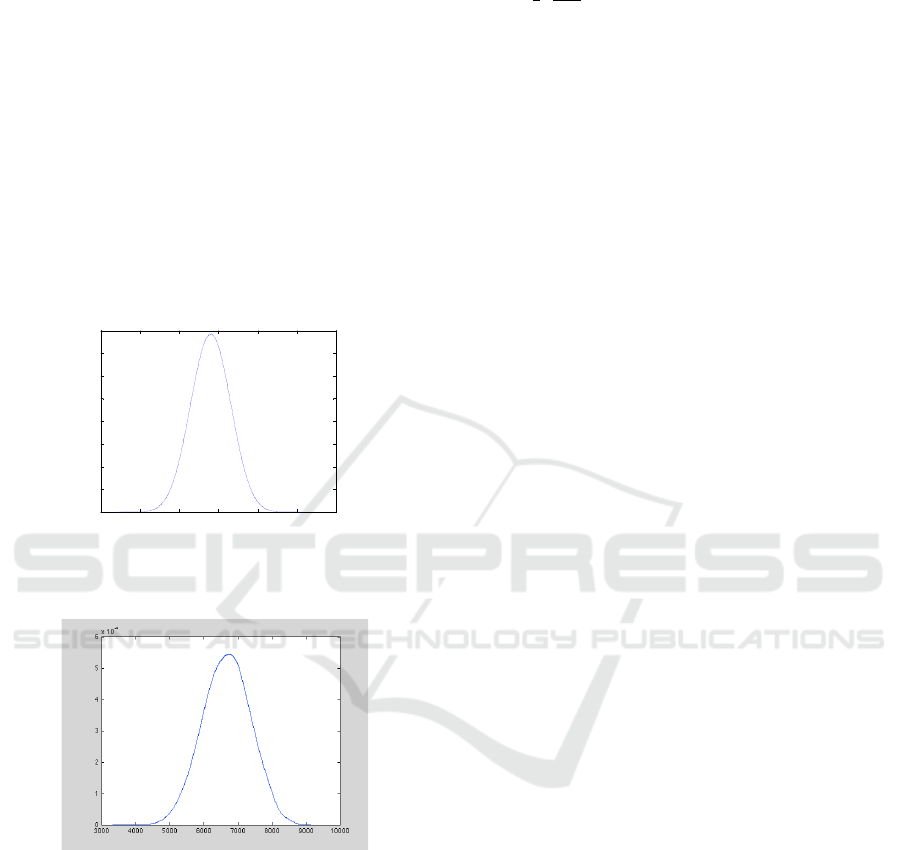
A typical probability distribution of all tour
lengths for a random TSP in a square unit is shown
in Fig. 1 where the total node number is 12. An ex-
ample of TSPLIB Burma14 is shown in Fig.2. Similar
results are observed for different total number of cities
for which all tour lengths can be obtained.
The organization of remaining parts of this paper
is: our major contributions are summarized in Sec-
tion 2, our methods are introduced in Section 3, and
Conclusions and future work are discussed in Section
4.
4 5 6 7 8 9 10
0
1
2
3
4
5
6
7
8
x 10
-3
Tour Lengths
Probability
Figure 1: The probability density of random 12-node TSP
in a squre unit.
Figure 2: The probability density of all tour lengths in
Burma14.tsp with 14 nodes.
2 RESULTS
The main contributions of this work can be summa-
rized as follows:
• We propose Generalized Beta (GB) distribution
as the probability density function of all tour
lengths distribution in a symmetric TSP in Eu-
clidean space (ESTSP), the four parameters of the
GB can be computed from given ESTSP data di-
rectly.
• For the first time, we introduce an iterative Trun-
cated GB (TGB) closed-form solution to obtain
(1+
1
2
(
α+1
α+2
)
K−1
)-approximation for a STSP where
K is the number of total iterations in TGB, and
α(>> 1) is the shape parameter of TGB and can
be determined once the TSP instance is given. The
result can approach the true optimum as K in-
creases.
3 METHODS
Firstly, a problem formulation and some preliminaries
are provided in this section.
3.1 Problem Formulation
Consider the n-node TSP defined in Euclidean space.
This can be represented on a complete graph G=
(V,E) where V is the set of vertices and E is the set of
edges. The cost of an edge (u, v) is the Euclidean dis-
tance (c
uv
) between u and v. Let the edge cost matrix
be C[c
i j
] which satisfies the triangle inequality.
Definition 1. Symmetric TSP (STSP) is TSP in Eu-
clidean distance (called ESTSP) and the edge cost
matrix C is symmetric.
Definition 2. 4STSP is a STSP whose edge costs are
non-negative and satisfies the triangle inequality, i.e.,
for any three distinct nodes (not necessary neighbor-
ing) (i, j,k), (c
i j
+c
jk
) ≥ c
ik
.
Definition 3. TSP tour. Given a symmetric graph G
in 2-dimensional Euclidean distance and its distance
matrix C where c
i j
denote the distance between node
i and j (symmetrically). A tour T has length
L =
N−1
∑
k=0
c
T (k),T (k+1)
(1)
where N is the total number of nodes in G and
T (N)=T (0) so that a feasible tour is formed.
Definition 4. The approximation ratio of an algo-
rithm. The ratio is the result obtained by the algorithm
over the optimum (abbreviated as OPT in this paper).
Observation 1. The probability density function of
all tour lengths in an ESTSP can be modelled by a
Generalized Beta (GB) distribution.
This is observed in Fig. 1 and other ESTSPs for
which we can obtain all tour lengths. More results are
provided in next section. This is also validated and
shown in (Vig and Palekar, 2008), where a scaled Beta
distribution is applied with scaled mean and scaled
variance. The author validated estimated results
by Anderson-Darling (A-D) test and Kolmogorov-
Smirnov (K-S) test for random TSP. They use these
ICORES 2017 - 6th International Conference on Operations Research and Enterprise Systems
282

estimates to fit various candidate distributions includ-
ing the Beta, Weibull and Normal cases, and conclude
that the (scaled) Beta distribution yields the best fit.
We further propose a Generalized Beta (GB) dis-
tribution. The probability density function (pdf) of
GB is defined as
f (x, α,β,A,B) =
(x −A)
α−1
(B −x)
β−1
Beta(α,β)
(2)
where Beta(α,β) is the beta function
Beta(α,β) =
Z
1
0
t
α−1
(1 −t)
β−1
dt, (3)
A and B is the lower bound and upper bound respec-
tively, α > 0, β > 0, see (Hahn and Shpiro, page 91-
98,126-128,1967). For TSP, A and B represents the
minimum and maximum tour length respectively.
The four central moments, mean (µ), variance,
skewness and kurtosis of the Generalized Beta distri-
bution with parameters (α, β, A, B) are given by:
µ = A + (B −A)
α
α + β
(4)
Var = (B −A)
2
αβ
(α + β)
2
(α + β + 1)
(5)
Skewness =
2(β −α)
p
1 + α + β
p
α + β(2 + α + β)
(6)
and Kurtosis
6[α
3
+ α
2
(1 −2β) + β
2
(1 + β) −2αβ(2 + β)]
αβ(α + β + 2)(α + β + 3)
(7)
The standard deviation is then given by
σ =
√
Var (8)
Once four central moments are known, or any four
parameters of (A, B, µ, Var, skewness, kurtosis) are
given, then four parameters of GB, i.e., (α, β, A, B)
can be determined easily from the four moments
match using Eqns.(4)-(7). When the problem size is
not large, the four central moments can be computed
exactly using methods proposed in (Stuffle 2009). As
the problem size increases, we can find any four pa-
rameters of (A, B, µ, Var, skewness) firstly, then find
four parameters of GB, i.e., (α, β, A, B).
For medium or large size problem, currently it is
not easy to find the fourth central moment. However,
the lower bound (A) can be easily computed by LKH
code (Helsgaun, 2009). So in the following sections,
we find four values (A, mean (µ), variance, skewness)
firstly, and then compute other parameters (B, α, β).
Firstly we introduce a method to compute maxTSP
(B) (Gutin and Punnen, 2002).
Definition 5. maxTSP. The maximum tour length (B)
is obtained using LKH where each edge cost (c
i j
) is
replaced by a very large value (M) minus the original
edge cost, i.e., (M-c
i j
). M can be set as the maximum
edge cost plus 1.
Since the characteristics of random TSP and TSPLIB
instances are different in Euclidean space, we intro-
duce the GB as the probability density function for
them separately.
3.2 GB as the Probability Density
Function for Random TSP
For medium size random TSP problems with n vary-
ing from 20 to 100, we can obtain four central mo-
ments easily (Suffle, 2009) and apply four moments
match to find four parameters for GB. After obtaining
four parameters, we then use linear regression to find
closed-form solution to (α, β) of GB for random TSP.
For n=20 to n=100, and we find that
α(n) = 1.9197n −32.166, R
2
= 0.9994 (9)
β(n) = 1.1168n −15.854, R
2
= 0.9982 (10)
A(n) = 0.6932
√
n + 0.8029,R
2
= 0.9956 (11)
B(n) = 0.7649n −0.6393, R
2
= 0.998 (12)
where R
2
is a measure of goodness-of-fit with value
between 0 and 1, the larger the better. We observe that
Eqns.(9)-(12) are highly accurate by extensive com-
putation results.
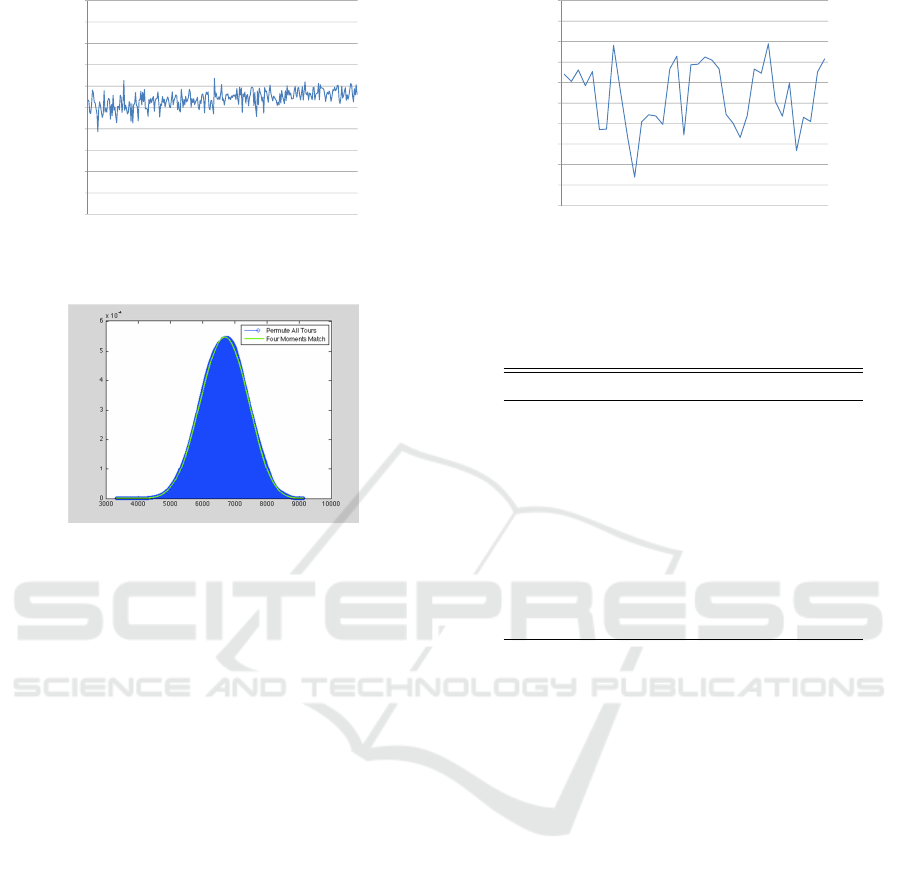
Observation 2. The relative errors between estimated
results (maxTSPs) by GB and LKH results are within
6.5% for random TSP.
The relative error is defines as (EstimatedValue-
OPT)/OPT×100%. We conduct tests for n=100 to
n=500. The results are shown in Fig.3 where LKH
is used to obtain maxTSP (B) results. We can observe
that the relative error between our results and LKH
are within 6.5% off the true optimums, with an aver-
age below 5%. Table 1 shows four parameters of GB
for random TSPs with n varying from 90 to 99.
3.3 GB as the Probability Density
Function for TSPLIB Instances in
Euclidean Distance
Firstly, we show an example of Burma14.tsp, which
we can permute its all tours and find that minimum
tour length (A) is 3233 and maximum tour length
(B) is 9139, Mean (µ)=6679, Variance=503064,
Skewness=-0.0632, Kurtosis=2.7972. Fig. 4 shows
exact result (in black color) by permuting all tour
A Near Optimal Approach for Symmetric Traveling Salesman Problem in Euclidean Space
283

0
0.01
0.02
0.03
0.04
0.05
0.06
0.07
0.08
0.09
0.1
Figure 3: The relative error between estimated results by
GB and OPT by LKH for Random TSP n=200 to 500.
Four Moments
Match Parameters:
A = 3233
B = 9579
α = 13.96
β= 11.79
Tour Lengths
Probability
Figure 4: The exact (Permute All Tours) and esti-
mated (Four Moments Match) probability distribution of
Burma14.tsp.
lengths and estimated probability density function
(in green color) by four central moment match with
(A=3233, B=9579, α=13.96,β=11.79). It can be ob-
served that two results match very well.
Observation 3. The relative error between the esti-
mated maximum tour lengths by GB and LKH results
is below 7% for medium size TSPLIB instances, with
an average below 5%.
We conduct tests by set n=14 to n=52 for which
the four central moments can be easily computed and
are given in (Stuffle 2009). Fig. 5 shows the relative
error between estimated results by GB and OPT by
LKH.
In Table 2 we show four parameters of GB for
TSPLIB with n varying from 14 to 52.
3.4 Truncated Generalized Beta
Distribution based on Christofides
Algorithm
Next, we introduce our algorithm, Truncated Gener-
alized Beta distribution Based on Christofides Al-
gorithm (TGB). TGB algorithm performs in seven
steps:
• (1). Finding the minimum spanning tree MST of
the input graph G representation of metric TSP;
-0.1
-0.08
-0.06
-0.04
-0.02
0
0.02
0.04
0.06
0.08
0.1
Figure 5: The relative error between estimated results by
GB and OPT by LKH for TSPLIB instances for n from 14
to 52.
Table 1: Four parameters of GB for some random TSP in-
stances.
n A(OPT) B α β
90 7.18 65.75 179.68 96.49
91 7.15 69.49 180.38 96.30
92 7.01 69.18 185.51 108.55
93 8.00 71.24 182.22 100.63
94 7.73 68.58 175.38 94.00
95 7.77 69.53 181.09 105.93
96 7.40 73.10 204.60 115.61
97 8.00 74.01 186.85 107.33
98 7.73 76.44 208.67 123.96
99 7.54 74.95 203.46 109.03
• (2). Taking G restricted to vertices of odd degrees
in MST as the subgraph G
∗
; This graph has an
even number of nodes and is complete;
• (3). Finding a minimum weight matching M
∗
on
G
∗
;
• (4). Uniting the edges of M
∗
with those of the
MST to create a graph H with all vertices having
even degrees;
• (5). Creating a Eulerian tour on H and reduce it
to a feasible solution using the triangle inequality,
a short cut is a contraction of two edges (i, j) and
( j,k) to a single edge (i,k);
• (6). Applying Christofides algorithm to a ESTSP
forms a truncated GB (TGB) for the probabil-
ity density function of optimal tour lengths, with
expectation (average) value at most 1.5OPT-ε,
where ε is a very small value; Applying k-opt to
the result of Christofides algorithm forms another
TGB for probability density function of optimal
tour lengths;
• (7). Iteratively apply this approach, taking the ex-
pectation value of (K −1)-th iteration as the upper
bound of the K-th iteration, we have the expecta-
tion value after K iterations (K ≥ 2).
ICORES 2017 - 6th International Conference on Operations Research and Enterprise Systems
284

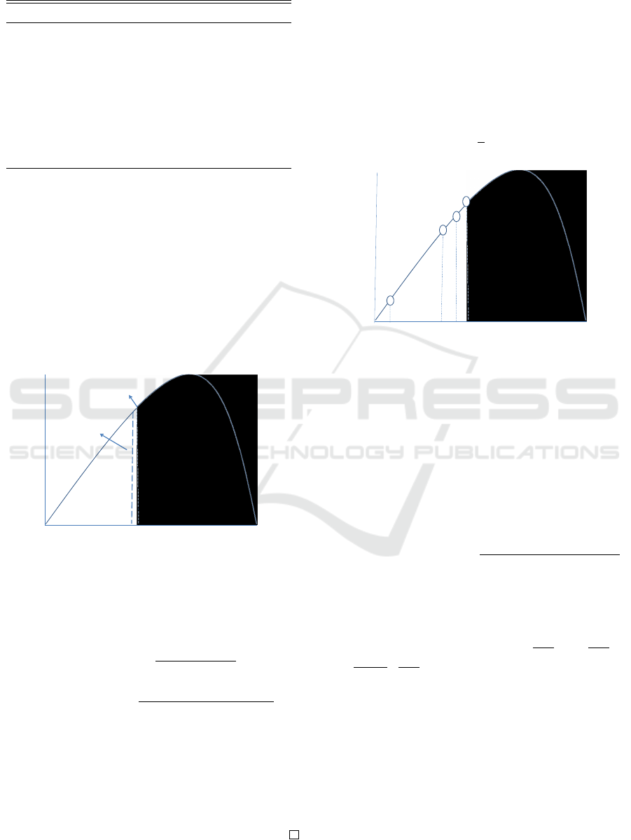
Table 2: Four parameters of GB for some TSPLIB in-
stances.
TSPLIB A(OPT) B α β
burma14 3323 9139 13.97 11.79
ulysses16 73.98 180.52 10.24 6.52
gr17 2085 6160 19.22 10.60
gr21 2707 10680 32.95 19.80
ulysses22 75.3 241.50 17.52 12.79
gr24 1272 4929 51.55 27.21
fri26 937 3681 28.87 16.91
bayg29 1610 6654 42.17 26.42
bays29 2020 8442 45.14 27.52
Lemma 1. Applying Christofides algorithm to a
ESTSP forms a truncated GB (TGB) for the proba-
bility density function of optimal tour lengths, with
expectation (average) value at most 1.5OPT-ε, where
ε is a very small value.
Proof. This is because that Christofides algorithm as-
sures that its result is at most 1.5OPT so that those
tours with lengths more than 1.5OPT are excluded
(truncated), as shown in Fig. 6 where tour lengths
larger than 1.5OPT (1.5A) are truncated in black
color.
B
A
1.5A1.5A-ε
Truncated
from above
The expectation
of TGB after
Christofides’ Alg
Figure 6: The Truncated GB by applying Christofides algo-
rithm.
The TGB in this case is truncated from above. Set
X as the variate of the GB, the probability density
function (pdf) of TGB is given by
f
1
t
(x,α,β,A,B, a,b) =
f (x, α,β, A,B)
Pr[a ≤ X ≤ b]
=
(x −A)
α−1
(B −x)
β−1
R
b
a
(x −A)
α−1
(B −x)
β−1
(13)
where a=A and b=1.5A. Therefore 1.5A is the upper
bound. We know that the average of Christofides al-
gorithm is at most 1.5OPT-ε (set as µ
1
t
) where ε is a
very small value, this is also validated in (Blaser et
al., 2012).
The four parameters of GB for some random TSP
and TSPLIB instances are provided in Table 1 and 2
respectively.
Definition 6. k-opt method. Local search with k-
exchange neighborhoods, also called k-opt, is the
most widely used heuristic method for the TSP. k -opt
is a tour improvement algorithm, where in each step k
links of the current tour are replaced by k links in such
a way that a shorter tour is achieved (see (Helsgaun,
2009) for detailed introduction).
In (Helsgaun, 2009), a method with computational
complexity of O(k
3
+ k
√
n) is introduced for k-opt.
BA
1.5A
2
3
K
1.5A-ε
1
Figure 7: The Iteratively Truncated GB.
Lemma 2. Applying k-opt to the result of
Christofides algorithm forms another TGB for prob-
ability density function of optimal tour lengths.
Proof. Applying k-opt to the result obtained by
Christofide algorithm as shown in Fig.7. The TGB
in this case is truncated from above. Denote the first
truncation by Christofides’ algorithm as the first trun-
cation (K=1). The probability density function of the
second TGB is given by
f
2
t
(x,α,β,A,B, a
2
,b
2
) =
(x −A)
α−1
(B −x)
β−1
R
b
2
a
2
(x −A)
α−1
(B −x)
β−1
(14)
In this case, a
2
=A, b
2
=1.5A because the distribu-
tion is based on the result after applying Christofides
algorithm which assures the upper bound is at
most 1.5A, see Fig.7. Setting ˆx=
x−A
B−A
, ˆa
2
=
A−A
B−A
=0,
ˆ
b
2
=
1.5A−A
B−A
=
0.5A
B−A
, we have
C
0
=
Z
b
2
a
2
(x −A)
α−1
(B −x)
β−1
dx
=
Z
ˆ
b
2
0
((B −A) ˆx)
α−1
((B −A)(1 − ˆx)
β−1
dx
= (B −A)
α+β−1
B
2
(0,
ˆ
b
2
,α,β) (15)
where
B
2
(0,t,α, β) =
Z
t
0
x
α−1
(1 −x)
β−1
dt (16)
A Near Optimal Approach for Symmetric Traveling Salesman Problem in Euclidean Space
285

By the definition of the expectation (mean) value (de-
noted as µ
2
t
) for f
2
t
(x,α,β,A,B, a
2
,b
2
), we have
µ
2
t
−A =
Z
b
2
a
2
(x −A) f
2
t
(x,α,β,A,B, a
2
,b
2
)dx
=
R
b
2
a
2
(x −A)
α
(B −x)
β−1
dx
C
0
=
(B −A)
α+β
B
2
(0,
ˆ
b
2
,α + 1,β)
C
0
= (B −A)
B
2
(0,
ˆ
b
2
,α + 1,β)
B
2
(0,
ˆ
b
2
,α,β)
=> µ
2
t
= A + (B −A)
B
2
(0,
ˆ
b
2
,α + 1,β)
B
2
(0,
ˆ
b
2
,α,β)
(17)
Taking the expectation value of (K −1)-th itera-
tion as the upper bound (
ˆ
b
K
=
µ
K−1
t
−A
B−A
) of the K-th
iteration, we apply this approach Iteratively and have
the expectation value after K iterations (K ≥ 2), de-
noted as µ
K
t
,
µ
K
t
= A + (B −A)
B
2
(0,
ˆ
b
K
,α + 1,β)
B
2
(0,
ˆ
b
K
,α,β)
= A + (B −A)g(
ˆ
b
K
)
Next we provide the proof for our main theorem.
Theorem 1. Applying TGB iteratively, we can obtain
quality-proved approximation, i.e., (1+
1
2
(
α+1
α+2
)
K−1
)-
approximation where K is the number of iterations in
TGB, α is the shape parameter of TGB and can be
determined or estimated once TSP instance is given.
Proof. Notice that the expectation value of the (K-1)-
iteration is taken as the upper bound (
ˆ
b
K
=
µ
K−1
t
−A
B−A
here A is OPT and B is the maxTSP) of the K-
iteration, as shown in Fig.7. Setting
g(
ˆ
b
K
) =
B
2
(0,
ˆ
b
K
,α + 1,β)
B
2
(0,
ˆ
b
K
,α,β)
(18)
The exact expression of g(
ˆ
b
K
) can be stated in a hy-
pergeometric series, and
B
2
(0,
ˆ
b
K
,α,β) =
ˆ
b
K
α
α
F(α,1 −β,α + 1,
ˆ
b
K
) (19)
and F(a,b, c,x)
= 1 +
ab
c
x +
a(a + 1)b(b + 1)
c(c + 1)2!
x
2
+
a(a + 1)(a + 2)b(b + 1)(b + 2)
c(c + 1)(c + 2)3!
x
3
+ ... (20)
In all cases, we have α >1, β >1,
ˆ
b
K
∈ (0, 1), there-
fore F(a,b, c,x) is an monotonic decreasing function.
We have
u
2
t
= A + (B −A)g(
ˆ
b
2
) ≤ A + 0.5A
α + 1
α + 2
(21)
continue this for g(
ˆ
b
3
), u
3
t
, g(
ˆ
b
4
), u
4
t
,..., so forth,
we have
ˆ
b
K
≤
0.5A
B −A
(
α + 1
α + 2
)
K−1
(22)
and
g(
ˆ
b
K
) =
B
2
(0,
ˆ
b
K
,α + 1,β)
B
2
(0,
ˆ
b
K
,α,β)
≤
α + 1
α + 2
ˆ
b
K
=
0.5A(
α+1
α+2
)
K−1
B −A
, (23)
Therefore
µ
K
t
= A + (B −A)
B
2
(0,
ˆ
b
K
,α + 1,β)
B
2
(0,
ˆ
b
K
,α,β)
= A + (B −A)g(
ˆ
b
K
)
≤ (1 +
1
2
(
α + 1
α + 2
)
K−1
)A, (24)
This means that, after the K-th iterative trunca-
tion, we can obtain the expectation value of (µ
K
t
)
which is close to the optimum (OPT=A) when K in-
creases. Actually, to make the approximation less
than C
0
, the TGB algorithm needs K to be at least
(1+
log2(C
0
−1)
log(1−1/(α+1))
).
Table 3 shows OPT, α, β, iteration numbers and
the approximation ratio (Appr) for TSPLIB instances
with n ≤ 600, where (α, β) are obtained (or esti-
mated) from (A, mean, variance, skewness) in Eqns
(4)-(7), and K is obtained in by TGB algorithm which
modifies LKH code. We observe that the TGB re-
sults are consistent with LKH OPT results in most
cases, there are only a few cases where TGB results
are few percentage difference from OPT, with 0.2%
off the true optimum on the average. For instance,
the difference is 7.8% for berlin52.tsp and 1.1% for
ulysses22.tsp. Our results are consistent with (Apple-
gate et al., 2003). These results validate Theorem 1.
Notice that LKH code performs very fast in practice
and our results are based on average performance.
4 CONCLUSIONS
In this paper, for the first time, we proposed GB and
Truncated Generalized Beta distribution (TGB) for
ICORES 2017 - 6th International Conference on Operations Research and Enterprise Systems
286

Table 3: Four parameters for some TSPLIB instances (n ≤
600).
α K-1 (1+0.5(
α+1
α+2
)
K−1
)A Appr
ulysses22 17.5 91 82.1 1.0042
berlin52 57.4 101 9052.4 1.0900
pr76 115.5 2451 108159.4 1.0000
rat99 128.1 1821 1219.2 1.0000
kroA100 137.3 3366 21285.3 1.0000
pr299 422.2 29117 48194.8 1.0000
lin318 563.1 39112 42042.4 1.0000
rd400 735.1 34936 15275.7 1.0000
d493 695.9 129767 35018.3 1.0000
rat575 892.03 84814 6796.36 1.0000
the probability distribution of optimal tour lengths in
a symmetric TSP in Euclidean space. Notice that our
TGB results are based on expectation (average) value
of probability distribution, which may be overesti-
mated for the number of iterations. In practice, LKH
algorithm performs very fast, with estimated compu-
tational complexity of O(n
2.2
) [9]. A few possible
research directions include:
• Improving the computational complexity. Cur-
rently the Christofides algorithm with minimum
perfect matching has computational complexity
O(n
3
). For large instances, this complexity should
be reduced.
• Find more efficient ways to compute especially
the third and fourth central moments of a given
TSP instance.
• Finding more applications. With closed-form
probability density function at hand, a lot of things
can be done better. For instance, computing more
statistical metrics, analyzing the average perfor-
mance of approximation algorithms and others.
ACKNOWLEDGEMENTS
This research is partially supported by China Na-
tional Science Foundation (CNSF) with project ID
61672136, 61650110513; and Xi Bu Zhi Guang
Project (R51A150Z10). A version of manuscript is
posted on http:/arxiv.orgpdf1502.00447.pdf
REFERENCES
D. Applegate, W. Cook, A. Rohe, Chained Lin-
Kernighan for large traveling salesman problems, IN-
FORMS Journal on Computing; Winter 2003; 15, 1;
ABI/INFORM Global pg. 82.
H. C. An, Robert Kleinberg, David B. Shmoys, Improving
Christofides Algorithm for the s-t Path TSP, 2012.
M. Blaser, K. Panagiotou and B. V. R. Rao, A Probabilis-
tic Analysis of Christofides’ Algorithm, Algorithm
Theory-SWAT 2012, Lecture Notes in Computer Sci-
ence Volume 7357, 2012, pp 225-236.
N. Christofides, Worst-case analysis of a new heuristic for
the travelling salesman problem, Report 388, Gradu-
ate School of Industrial Administration, CMU, 1976.
W. Cook, In Pursuit of the Traveling Salesman, Princeton
University Press, 2012.
In G. Gutin and A. Punnen, editors, The Traveling Sales-
man Problem and its Variations, Chapter 1 The Maxi-
mum Traveling Salesman Problem, Kluwer Academic
Publishers, New York, NY, USA, 2002.
B. L. Golden. Closed-form statistical estimates of optimal
solution values to combinatorial problems. In ACM
78: Proceedings of the 1978 annual conference, pages
467-470, New York, NY, USA, 1978. ACM.
G. J. Hahn and S. S. Shpiro, Statistical Models in Engineer-
ing, John Wiley & Sons, Inc., New York, 1967.
K. Helsgaun, General k-opt submoves for the Lin-
Kernighan TSP heuristic. Mathematical Programming
Computation, 2009,doi: 10.1007/s12532-009-0004-6.
D. S. Johnson, L. A. McGeoch, The Traveling Salesman
Problem: A Case Study in Local Optimization, Lo-
cal search in combinatorial optimization 1, 215-310,
1998.
D. S. Johnson, The Traveling Salesman Problem for ran-
dom points in the unit square: An experimental and
statistical study. Technical Report, 2014.
E. Klarreich, Computer Scientists Find New Shortcuts
for Infamous Traveling Salesman Problem, SIMONS
SCIENCE NEWS, Jan. 29, 2013.
S. Lin, B. W. Kernighan, An effective heuristic algorithm
for the traveling-salesman problem. Oper. Res.21,
498-516 (1973).
LKH codes, http://www.akira.ruc.dk/ keld/research/LKH/,last
accessed Jan. 15th of 2015.
G. Reinelt. TSPLIB, a traveling salesman problem library.
ORSA Journal on Computing, 3(4):376-384, 1991.
S. Reiter and D. B. Rice. Discrete optimizing solution
procedures for linear and nonlinear integer program-
ming problems. Management Science, 12(11):829-
850, 1966.
P. J. Sutcliffe, Moments over the Solution Space TSP, PhD
Thesis, University of Technology, Sydney, 2009.
V. Vig and U. S. Palekar. On estimating the distribu-
tion of optimal traveling salesman tour lengths using
heuristics. European Journal of Operational Research,
186(1):111-119, April 2008.
J. Vygen, New approximation algorithms for the TSP,
OPTIMA 90 (2012), 1-12.
A Near Optimal Approach for Symmetric Traveling Salesman Problem in Euclidean Space
287