Matching of Line Segment for Stereo Computation

O. Martorell, A. Buades and B. Coll

Dpt. Mathematics and Computer Science, Universitat de les Illes Balears,

carret. Valldemossa, km 7,5, 07122 Palma, Spain

Keywords:

Stereo, Matching, Segments, Diffusion, T-junction, Convexity Points.

Abstract:

A stereo algorithm based on the matching of line segments between two images is proposed. We extract

several characteristics of the segments which permit its matching across the two images. A depth ordering

computed from the line segments of the reference image allows us to attribute the match disparity to the

correct pixels. This depth sketch is computed by joining close line segments and identifying T-junctions and

convexity points. The disparity computed for segments is then extrapolated to the rest of the image by means

of a diffusion process. The performance of the proposed algorithm is illustrated by applying the procedure to

synthetic stereo pairs.

1 INTRODUCTION

The human visual system has the ability to infer the

depth of a scene from the two images captured by the

eyes. Our brain is responsible for merging the infor-

mation from the 2D images in order to determine the

depth ordering of objects in scene. This process is

called stereopsis.

The computation of the depth of objects in a scene

is one of the main problems in computer vision. The

computation of such depth has been an intensive re-

search area. If the images are stereo rectiﬁed, mean-

ing that the epipolar lines are both horizontal, the

computation of the distance between the observer and

each 3D point, reduces to the computation of the dis-

parity or difference of horizontal coordinates of the

same point in both images.

Numerous algorithms have been proposed in or-

der to compute correspondences between points in

both images. The main classiﬁcation separates lo-

cal from global algorithms (Scharstein and Szeliski,

2002). Local algorithms match a small window

around each pixel with the most similar window in

the same epipolar line in the second image. Only dis-

tinctive patches can be matched correctly. Small win-

dows without texture or geometry are matched am-

biguously, and therefore matches are discarded. The

most common metrics for this window matching are

based on correlation, intensity differences, and rank

metrics (Tombari et al., 2008). Recent methods adapts

the shape and size of the window to the image content

itself. Windows are preferred to contain only pixels

with the same disparity (Buades and Facciolo, 2015;

Hirschm

uller et al., 2002) or at least belonging to the

same physical object (Patricio et al., 2004; Yoon and

Kweon, 2006; Wang et al., 2006; Rhemann et al.,

2011).

We ﬁnd local algorithms matching features as

edge segments or contours. These methods are fea-

ture based instead of intensity based, see for in-

stance (Brown et al., 2003) for a review. Even if

feature based matching is less popular than intensity

based, there’s a prominent literature in the ﬁeld. In

(Nasrabadi, 1992), a stereo matching algorithm based

on the generalized Hough transform of small edge

segments had proposed. In the same line, Ma, Si

and Chen (Ma et al., 1992) utilized a curve based ap-

proach to perform matching by assuming that quadric

based curves exist on the surfaces of the objects in

the scene. Robert and Faugeras (Robert and Faugeras,

1992) approximated edge contours as B- splines and

use these as their matching primitives. In (McCane

and de Vel, 1994), the authors presented a stereo

algorithm based on the matching of free-form con-

tours. This matching process was proposed as a near-

est neighbor problem by using a set of features ex-

tracted from each of the contours.

In contrast to local methods, global methods aim

to determine disparities for all reference image pix-

els at once (Szeliski et al., 2008). This is achieved by

minimizing an energy function composed of a corre-

spondence data term and a regularization term. The

410

Martorell O., Buades A. and Coll B.

Matching of Line Segment for Stereo Computation.

DOI: 10.5220/0006121004100417

In Proceedings of the 12th International Joint Conference on Computer Vision, Imaging and Computer Graphics Theory and Applications (VISIGRAPP 2017), pages 410-417

ISBN: 978-989-758-227-1

most commonly used optimization methods for mini-

mization of energy functions are based on graph cuts

(Kolmogorov and Zabih, 2001) and belief propaga-

tion (Sun et al., 2003). Global methods depend on ad-

ditional parameters difﬁcult to ﬁx in general, its value

being different for each stereo pair.

Finally, monocular algorithms are also proposed

in the literature. These algorithms use a single im-

age to infer the depth ordering of objects in the

scene. Making use of a single image, these algorithms

can not estimate the actual depth of the objects but

only which are further or closer. These methods are

based on the computation of T-junctions, convexity

clues and occlusion detection (Dimiccoli et al., 2008;

Calderero and Caselles, 2013; Palou and Salembier,

2013). The algorithm in (Dimiccoli et al., 2008) de-

tects local depth cues based on the response of a line

segment detector LSD, (Grompone von Gioi et al.,

2010). The LSD method is aimed at detecting lo-

cally straight contours on images by using a contrario

validation approach according to Helmholtz princi-

ple. This algorithm joins the Burn’s segment detector

(Burns et al., 1986) with a contrario validation tech-

niques (Desolneux et al., 2000).

In this work, we propose a feature matching al-

gorithm for depth estimation from a stereo pair. We

match line segments across the two images to obtain

a disparity estimate for points belonging to these seg-

ments. Being segment points at the boundary between

two different objects, it is not clear from the segment

description which pixels in the image should have

the estimated disparity. We use the monocular depth

sketch obtained with (Dimiccoli et al., 2008) to re-

move this ambiguity and give the computed estimate

to the closer object. This local depth information de-

ﬁned only on the segments is extrapolated to all the

pixels of the image by applying a non-linear diffusion

process.

The rest of the paper is organized as follows. Sec-

tion 2 introduces the LSD algorithm (Grompone von

Gioi et al., 2010). In Section 3 we describe the

monocular algorithm proposed in (Dimiccoli et al.,

2008). Section 4 presents the proposed algorithm for

stereo matching. In Section 5 we show a set of experi-

ments to validate the proposed algorithm followed by

the conclusion n Section 6.

2 LINE SEGMENT DETECTION

ALGORITHM

In this section we describe the LSD algorithm for de-

tecting line segments introduced by (Grompone von

Gioi et al., 2010), (Grompone von Gioi et al., 2012).

In practice, the LSD algorithm takes a gray-level im-

age as input and returns a list of detected line seg-

ments.

First of all, the algorithm computes a unit vector

ﬁeld for each pixel of the image, called the level-line

angle, such that all vectors are tangent to the level line

going through their base point. That produces a vec-

tor ﬁeld in all the image. Then, the vector ﬁeld is

segmented into connected regions of pixels that share

the same level-line angle up to a threshold parame-

ter. These connected regions of vector ﬁelds are called

line support regions. At this point, each line support

region is a candidate for a line segment. The main

rectangle direction is taken as the principal inertial

axis of the line support region. In order to validate or

not the rectangle as a detected line segment, the total

number of pixels in the rectangle, n, and its number

of aligned points, k, are used.

The validation process is based on the a contrario

approach and the Helmholtz principle. This princi-

ple states that no perception (or detection) should be

produced on an image of noise. Then, an event is

validated if the expected number of events as good

as the observed one is small on the a contrario model.

Then, a number of false alarms (NFA) associated with

a rectangle r, gives us the lower bound for the valida-

tion of r.

More concretely, the steps of the algorithm are the

followings:

• The image gradient is computed at each pixel us-

ing a 2 × 2 mask by applying a difference scheme

and using a threshold ρ which depends of the an-

gle tolerance to be used in the region growing al-

gorithm.

• Pixels are classiﬁed into the bins according to

their gradient magnitude which correspond to the

more contrasted contours. A threshold is used for

accepting or rejecting the gradient magnitude.

• Starting from a seed pixel in the ordered list of un-

used pixels, a region growing algorithm is applied

to form a line-support region.

• A rectangle associated to a line-support region

must be found. The center of mass of the region is

selected as the center of the rectangle and the main

direction of the rectangle is set to the ﬁrst inertia

axis of the region. For the width and length of

the rectangles, the parameters are set to the small-

est values that make the rectangle to cover the full

line-support region.

• The pixels in the rectangle whose level-line angle

is equal to the main direction, up to a tolerance pπ,

are called p-aligned points. If the total number

of pixels in the rectangle is denoted by n and the

Matching of Line Segment for Stereo Computation

411

number of p-aligned points is denoted by k, then,

then the number of false alarms (NFA) associated

with the rectangle r is computed in the form

NFA(r) = (NM)

5/2

γB(n,k, p),

where N and M are the number of columns and

rows of the image and B(n, k, p) is the binomial

tail

B(n,k, p) =

∑

j=k





(1 − p)

n− j

Finally, only the rectangles with a NFA less than

a threshold are validated as a detections.

Figure 1: On the left, original image. On the right, the de-

tected segments by applying the LSD algorithm.

3 RELATIVE DEPTH ORDER IN

A SIMPLE IMAGE

In the ﬁeld of computer vision, the monocular depth

estimation problem tries to extract the depth order of

the objects present in a scene using only information

from a single view or image. Since this information

is partial, in general, the extracted depth relations are

relative in the sense that we can not deduce the abso-

lute depth position of an object in the scene.

In this section, we describe the method (Dimic-

coli et al., 2008) that we will use with minor modiﬁ-

cations. The algorithm estimates the occlusions (be-

tween overlapping objects) and convex contours of

objects. From this low-level features, the depth or-

dering is computed.

For the estimation of the occlusions and convex

contours, we use the list of detected segments of the

image computed from the LSD algorithm. From that,

we found all possible local conﬁgurations of the seg-

ments which allow us to detect the T -junctions and

the convexity points. Remember that a T -junction

conﬁguration is formed by the conﬂuence of the

boundary of two different objects and the intersection

point is called a T -junction point. Based on the set of

segments of the image, we deﬁne a T -junction point a

point where meet the ends of three different segments

or two segments, and the latter case, only one of them

by the end. By the contrary, a convexity point is a

point where meet the ends of two different segments

and with different slope.

3.1 Algorithm for the T -junction and

Convexity Points Estimation

From the set S = {s

,. .. ,s

} of detected segment by

applying the LSD algorithm, the output parameters

are the ends segment points, (x

) and (x

) and

the angle of the slope, θ

, i = 1, .. ., n. Note that we

can deﬁne a lexicographic order on the ends segment

points by the following rule: (x

) ≤ (x

) if and

only if x

< x

and y

< y

if x

= x

Given two different segments, we deﬁne the fol-

lowing rules to decide their relative position.

a) Intersection point: we call X the point of inter-

section of the straight lines which contain the two

segments.

b) Proximity of the segments to the intersection

point: we say that a segment s is near the point of

intersection X if one of the following conditions

holds:

b.1) the end nearest of s to X , ( ¯x, ¯y), satisfy that

the distance d(( ¯x, ¯y),X) is lesser than a certain

threshold.

b.2) the point X belongs to s.

c) Relative position of the segments s

and s

to be

part of a convexity or T -junction: the difference of

the angles |θ

− θ

| must be greater than a certain

threshold.

d) Parallel segments: two segments s

and s

, with

ends segment points, (x

) and (x

), l = 1,2,

are parallel if the difference |θ

− θ

| is smaller

than a given threshold. Furthermore, the point of

intersection X must be the midpoint between the

end points (x

) and (x

) or between (x

)

and (x

). In both cases, these ends points are

the ends closer.

From these rules, we can deﬁne the algorithm to

search T -junction and convexity points.

• A point X is a T -junction point if satisﬁes one of

the following conditions:

I) In the case of three different segments, it must

be fulﬁlled the following two conditions:

i1) There exist two segments s

and s

, with

intersection point X, satisfying conditions a),

b1) and c); or conditions a), b1) and d).

i2) There exist another segment s

satisfying

b1), with respect to X , and c), with respect to

and s

VISAPP 2017 - International Conference on Computer Vision Theory and Applications

412

II) In the case of two different segments, it must

be fulﬁlled the following two conditions:

i3) There exist two segments s

and s

, with

intersection point X, satisfying conditions a),

b2) and c).

i4) If X belongs to s

, then the distance of the

end nearest of s

to X must be greater than a

certain threshold and the distance of the end

nearest of s

to X must be lesser than a given

threshold.

• A point X is a convexity point if there exist two

segments s

and s

, with intersection point X, sat-

isfying conditions a), b1) and c).

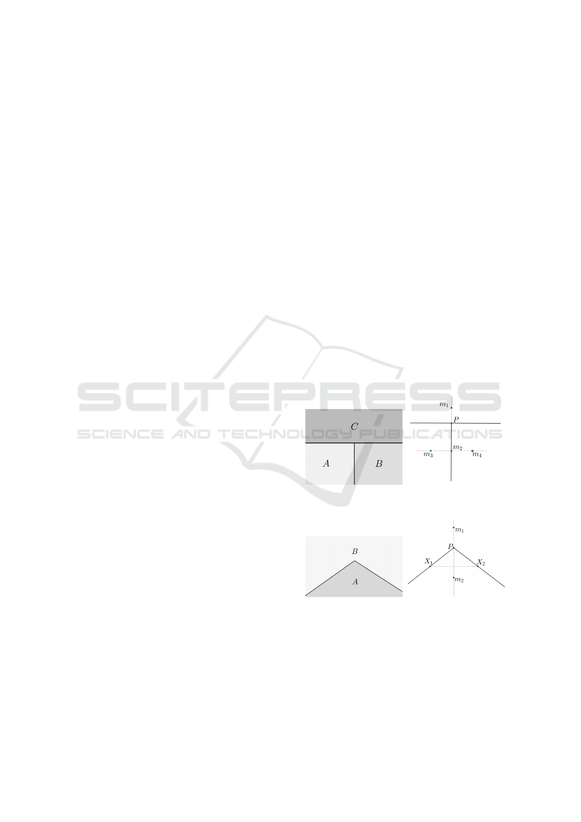
3.2 Computation of the Depth

Once calculated the T -junction and convexity points,

the conﬁguration of its neighborhood allows us to

classify the type of singularity. In most situations the

T -junction conﬁguration is formed when two sets A

and B are occluded by a third one C. That means the

neighborhood of the singularity is segmented by three

different regions where region A and B are behind and

C is in front. By the contrary, in the convexity conﬁg-

uration, only two regions A and B are determined in

a neighborhood of the singularity.

Let us take a point representative of each of these

regions and assign labels depending on whether the

region is in front (FSP: Foreground Source Point) or

behind (BSP: Background Source Point). In addition,

each label is assigned a numerical value which then

will allow us to extrapolate information from these

points to the other parts of the image using a diffusion

ﬁltering.

For the T-junction conﬁguration, we take the

points m

, m

and m

that represent each region and

are calculated as follows: ﬁrst we determine the seg-

ment s that separates the regions A and B and compute

the points m

and m

, which are at the same distance

from the center of the T-junction P and on the straight

line containing s. In this way, thus m

is inside C and

is on s. Now we calculate m

and m

: they are in

the perpendicular direction to s passing per m

and at

the same distance from m

, see Figure 2. Since A and

B are behind and C is in front, m

is labeled as FSP

while m

and m

are labeled as BSP.

In the case of convexity conﬁguration, we choose

the points m

and m

that represent each region and

are calculated as follows: take the points X

and X

which are located on each of the segments and at the

same distance d of the point of intersection of the

two segments P. Then, we choose m

and m

on the

straight line perpendicular to the line joining X

and

and at the same distance from P, see Figure 3. In

this case, due to the convexity conﬁguration, we as-

sign m

and m

the labels BSP and FSP, respectively.

The recovery of the relative depth order on the im-

age is achieved by global integration of these local

depth information from the same object by applying a

non-linear diffusion ﬁltering, the Depth Diffusion Fil-

ter (DDF), see (Dimiccoli et al., 2008). To do that, we

consider z(x) the depth value of pixel x. We initialize

as z(x) = 1 the points labeled as FSP while the other

points (labeled as BSP and not labeled) are initialized

as z(x) = 0. Then we apply the DDF:

DDF

r,δ

z(x) = max

y∈B

(x)

z(y) · w(x, y), (1)

where

w(x,y) =



1 si |I(x) −I(y)| ≤ δ,

0 si |I(x) −I(y)| > δ.

In the application of this diffusion ﬁlter, we need

an additional constraint for the separation of the ob-

jects. In fact, the points labeled as BSP and FSP,

which are in neighboring regions, are related because

we want to preserve the different depth in the inter-

polation process. To do that, we impose that the dif-

ference absolute value between each pair of BSP and

FSP is greater than 1. In Figure 4 we give an example

of the application of the algorithm.

Figure 2: On the left, the T -junction conﬁguration. On the

right, the starting points for the depth computation.

Figure 3: On the left, the convexity point conﬁguration. On

the right, the starting points for the depth computation.

4 STEREO MATCHING

ALGORITHM

We propose an algorithm for computing line segment

correspondences between two images of a stereo pair.

Matching of Line Segment for Stereo Computation

413

Figure 4: On the left, the original image where the three

polygons overlap with each other. On the right, the result

after applying the algorithm. The black color corresponds

to the value of depth three, thus making the rectangle on the

right is ahead of the rest. Furthermore, how strong is gray,

the greater the depth value.

We assume that the images are rectiﬁed in epipolar

geometry. We associate to each segment a descriptor

containing several characteristics of it. A cost func-

tion is deﬁned to compare two segments based on

their characteristics. For each segment in the refer-

ence image, the segment in the second image match-

ing with minimum cost is selected.

4.1 Matching Segments

We extract the following features from each segment:

c(1) length of the segment,

c(2) angle of the slope of the segment,

c(3) y-coordinate of the centroid of the segment,

c(4) x-coordinate of the centroid of the segment,

c(5) contrast sign of the segment, which is given by

the sign of the majority of pixels that belong to the

segment. By deﬁnition, sign(x,y) = sign(I(x , y)−

I(x +1,y)), where I is the grey level image.

In order to reduce ambiguity in the segment

matching between images I

and I

, we start discard-

ing those matches which do not agree with the epipo-

lar restriction or would have a too large disparity com-

pared to the camera motion. We apply the following

criteria:

• From the epipolar assumption, if the difference

of the y-centroids between the segment s

of I

and the segment s

of I

is greater than a certain

threshold (in practice 5), then we discard the cor-

respondence between s

and s

• Assuming we have some knowledge about the dis-

placement of the camera and from the epipolar

assumption, we also discard the correspondences

between s

and s

if the difference of their x-

centroids is greater than a certain threshold.

• If the difference between the angles of the seg-

ments s

and s

is greater than a certain threshold

(in practice π/10), then we discard the correspon-

dence between s

and s

• We also discard the correspondence of a pair of

segments having a different sign contrast.

For the remaining possible correspondences, we com-

pute a cost for each match depending on the charac-

teristics c(k), k = 1, 2,3.

We denote by c

(k), k = 1,··· , 3 the features of

the indexed segment s

from the left image and by

r j

(k), k = 1,··· ,3 the features of the indexed seg-

ment s

from the right image. Then the cost function

to match segment s

with segment s

is deﬁned as

C(i, j) =

∑

k=1



(k) −c

r j

(k)



where the weights W

, k = 1,2,3, gives more impor-

tance to certain features. Note that for a given seg-

ment s

of the left image, min

C(i, j) is reached for

some s

, where s

is a segment of the right image.

Then, we put in correspondence segment s

with seg-

ment s

4.2 Computation of the Disparity Map

Once segment correspondences are estimated we as-

sociate a disparity value to each pixel of the segment.

For a given segment s

, suppose that s

is the corre-

spondence segment. Let d

= x

−x

and d

= x

−x

be the difference between the x -coordinate of both

ends of the paired segments. The disparity value of

all pixels (x,y) of s

is given by

(x,y) = (d

− d

) · L(x, y) + d

, (2)

being

L(x,y) =

(x − x

)

+ (y − y

)

− x

)

+ (y

− y

)

That is, the estimated disparity varies linearly be-

tween the disparity of the two end points.

Being a segment the boundary between two ob-

jects, the disparity given to the segment actually is

due to the motion of the occluding object. That is, we

must give this disparity only to pixels belonging to the

occluding object. We use at this point the depth order-

ing computed from the reference image as described

in Section 3.

• Compute the monocular depth for the reference

image.

• For each pixel of the segment, we give the esti-

mated disparity computed in (2) to the neighbor-

ing pixels which are closer to the observer. We

use a mask M to identify pixels (x, y) for which

an estimate was given, M (x,y) = 1. Otherwise,

M(x,y) = 0.

VISAPP 2017 - International Conference on Computer Vision Theory and Applications

414

Finally, an iterative diffusion process assigns for a

given pixel, the average of the disparity values of its

neighboring pixels, called Average Depth Diffusion

Filter (ADDF). This average updates only the value

of pixels for which the disparity was not estimated by

the matching process. That is, the values computed

by the segment matching process are maintained con-

stant during the whole process permitting its diffusion

to the rest of pixels. Speciﬁcally, we apply the ﬁlter

ADDF

r,δ

d(x, y) =

∑

(i, j)∈B

(x,y)

d(i, j) · w(x,y,i, j),

(3)

for pixels with M(x, y) = 0, while originally estimated

pixels are not modiﬁed, d(x,y) = d

(x,y) if M(x,y) =

1. The weight distribution averages pixels expected to

belong to the same object,

w(x,y,i, j ) =



1 si |I

(x,y) −I

(i, j)| ≤ δ,

0 si |I

(x,y) −I

(i, j)| > δ,

and W =

∑

(i, j)∈B

(x,y)

w(x,y,i, j ). In practice, the val-

ues of δ and r are ﬁxed to 5 and 3, respectively.

5 EXPERIMENTS

In this section a series of test ﬁgures are examined in

order to provide more intuition and understanding of

the proposed method.

First of all, we want to note that for displaying the

disparity on the corresponding image, there is a differ-

ence on the background color of the output disparity

image.

• When the background color is white, all objects

have moved to the left with respect to their posi-

tion in the reference image. And the closer the

level of gray to black, the displacement has been

greater.

• When the background color is black, all objects

have moved to the right with respect to their po-

sition in the reference image. And the closer the

level of gray to white, the displacement has been

greater.

• When the background color is gray level, there ex-

ist objects that have been moved in one direction

or the other. More concretely, objects with color

close to white are shifted to the right and objects

with color close to black, to the left.

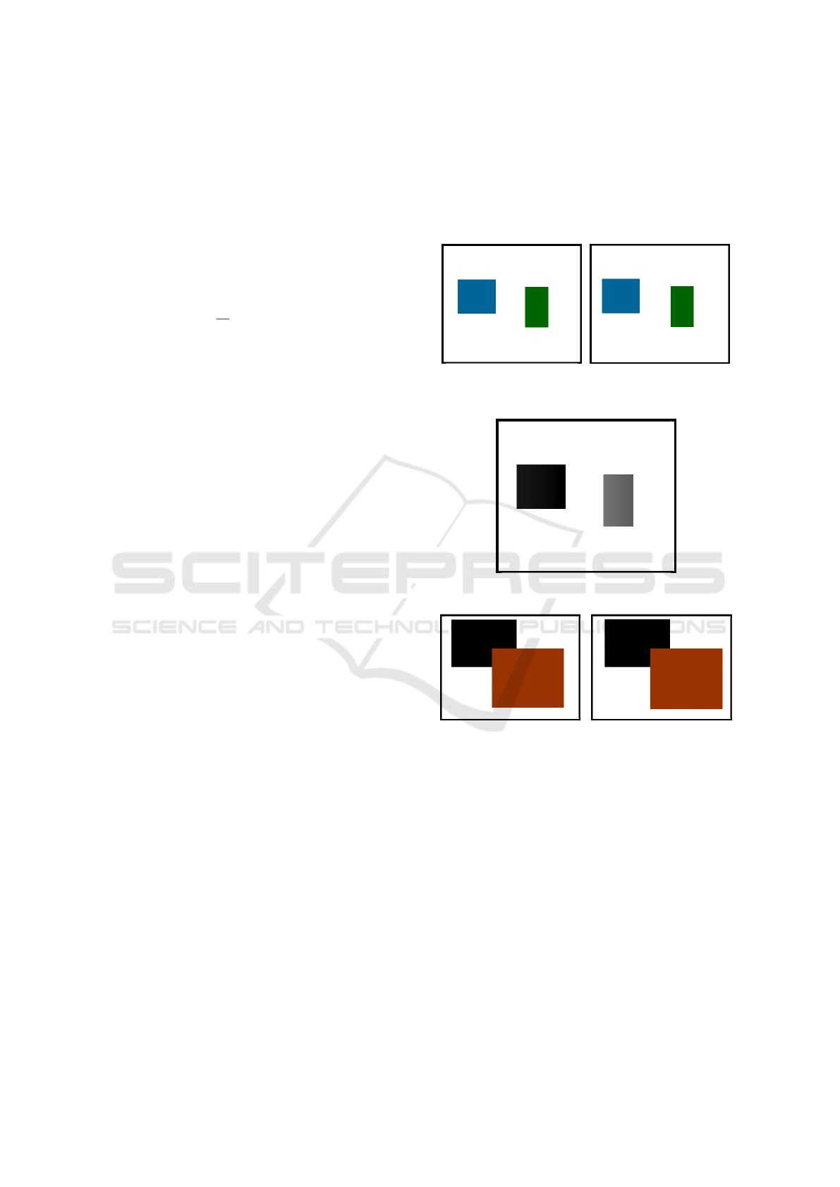
Figure 5 is an example of a pair of stereo images

consisting of two rectangles. The displacement of

each rectangle is different from the other, but the two

movements are uniform. The result is given in Figure

6. The fact that the color is different comes from each

rectangle has moved a different distance and therefore

have a different disparity value. As a consequence,

we can deduce that the blue rectangle is the closest to

the eye or the camera, because it is what is associated

with a greater displacement.

Figure 5: An example of a pair of stereo images with two

rectangles non-overlapping.

Figure 6: The result of the disparity map.

Figure 7: An example of a pair of stereo images consisting

of two overlapping rectangles.

Figure 7 is an example of a pair of stereo images

consisting of two overlapping rectangles that have

moved in the same direction. As in previous example,

the displacement of each rectangle is different from

the other, but the two movements are uniform. Figure

8 shows the ﬁnal result. Because the background is

black, the two objects have been moved to the right

with respect to its position in the reference image and

the rectangle in front has moved more than the other.

In the following experience, the displacement of

the objects is not uniform, see Figure 9. From the al-

gorithm we get that each segment that makes up the

border of the object tends to have a different dispar-

ity. Applying the ﬁlter DDF (1), the result is a jump

disparity between neighboring pixels. However, if we

Matching of Line Segment for Stereo Computation

415

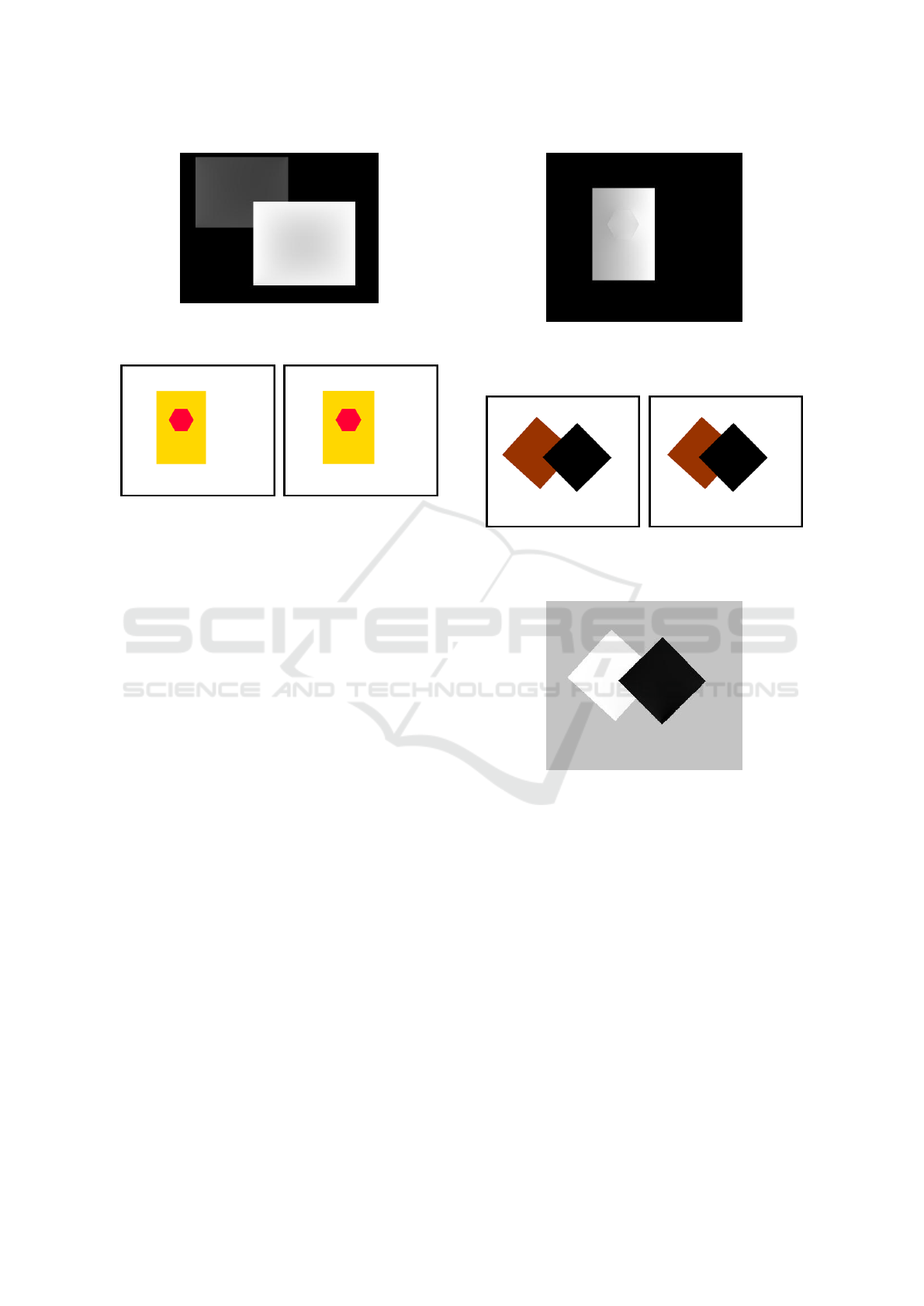
Figure 8: The disparity map after applying our proposed

algorithm to the pair of images of Figure 7.

Figure 9: The pair of stereo images where we suppose that

the displacement of the object is not uniform.

use the averaging ﬁlter ADDF (3), then the disparity

is gradually increased, thus causing the grow of the

disparity value is more smooth and continuous from

one border to another one of the polygon. Figure 10

shows the result by the application of the algorithm

to Figure 9. We can see that the gray level increases

from left to right, as the object is displaced in a uni-

form manner. Speciﬁcally, the left side has had a dis-

placement greater than the right side. This example

justiﬁes the use of an interpolation method for calcu-

lation of disparity in all the points of a segment: if we

didn’t use this method, the algorithm would give us

the same disparity for all points of the segment, when

really every point of the segment has a different dis-

placement.

Finally, we present an experiment given by the

movement of two rectangles but the polygons are not

parallel to the horizontal axis, which gives lead to ge-

ometrical shape of a rhombus. In addition, each poly-

gon is moving in a different direction, see Figure 11.

Applying the algorithm, we can show the disparity

map on Figure 12. We can observe that each rect-

angle has moved in a different direction and the black

rectangle is closer as it has a greater disparity.

6 CONCLUSIONS

The aim of this work has been to propose a feature

matching algorithm for the stereo vision problem by

using the segments of the image. The experimental

Figure 10: The result of the disparity map. We can see that

the left side has had a displacement greater than the right

side.

Figure 11: The pair of stereo images where the main seg-

ments of the T -junctions are not parallel to the the horizon-

tal axis.

Figure 12: The result of the disparity map. We observe that

each rectangle has moved in a different direction and the

black rectangle is closer as it has a greater disparity.

tests indicate that results are promising for both uni-

form and non-uniform movements and geometric im-

ages.

The future work includes the application of this

algorithm to real stereo pairs and the use of curves

additionally to line segments.

ACKNOWLEDGEMENTS

This work has been partially supported by the Minis-

terio de Ciencia e Innovaci

on of the Spanish Govern-

ment under grant TIN2014-53772-R.

VISAPP 2017 - International Conference on Computer Vision Theory and Applications

416

REFERENCES

Brown, M. Z., Burschka, D., and Hager, G. D. (2003). Ad-

vances in computational stereo. IEEE Trans. Pattern

Anal. Mach. Intell., 25(8):993–1008.

Buades, A. and Facciolo, G. (2015). Reliable multiscale

and multiwindow stereo matching. SIAM Journal on

Imaging Sciences, 8(2):888–915.

Burns, J., Hanson, H. R., and Riseman, E. M. (1986). Ex-

tracting straight lines. EEE Transactions on PAMI,

8(4):425–455.

Calderero, F. and Caselles, V. (2013). Recovering rela-

tive depth from low-level features without explicit t-

junction detection and interpretation. Int. J. Comput.

Vision, 104(1):38–68.

Desolneux, A., Moisan, L., and Morel, J. (2000). Mean-

ingful alignments. International Journal of Computer

Vision, 40(1):7–23.

Dimiccoli, M., Morel, J.-M., and Salembier, P. (2008).

Monocular depth by nonlinear diffusion. In Proceed-

ings of the 2008 Sixth Indian Conference on Computer

Vision, Graphics & Image Processing, ICVGIP ’08,

pages 95–102, Washington, DC, USA. IEEE Com-

puter Society.

Grompone von Gioi, R., Jakubowicz, J., Morel, J., and G.,

R. (2010). Lsd: A fast line segment detector with a

false detection control. IEEE Transactions on Pattern

Analysis and Machine Intelligence, 32(4):722–732.

Grompone von Gioi, R., Jakubowicz, J., Morel, J.-M., and

Randall, G. (2012). LSD: a Line Segment Detector.

Image Processing On Line, 2:35–55.

Hirschm

uller, H., Innocent, P. R., and Garibaldi, J. (2002).

Real-time correlation-based stereo vision with re-

duced border errors. International Journal of Com-

puter Vision, 47(1-3):229–246.

Kolmogorov, V. and Zabih, R. (2001). Computing vi-

sual correspondence with occlusions using graph cuts.

In Computer Vision, 2001. ICCV 2001. Proceedings.

Eighth IEEE International Conference on, volume 2,

pages 508–515. IEEE.

Ma, S. D., Si, S. H., and Chen, Z. Y. (1992). Quadric curve

based stereo. In ICPR 92, pages 1–4. IEEE.

McCane, B. J. and de Vel, O. (1994). A stereo matching

algorithm using curve segments and cluster analysis.

Technical report, Citeseer.

Nasrabadi, N. M. (1992). A stereo vision technique using

curve-segments and relaxation matching. IEEE Trans.

Pattern Anal. Mach. Intell., 14(5):566–572.

Palou, G. and Salembier, P. (2013). Monocular depth or-

dering using t-junctions and convexity occlusion cues.

IEEE transactions on image processing, 22(5):1926–

1939.

Patricio, M. P., Cabestaing, F., Colot, O., and Bonnet, P.

(2004). A similarity-based adaptive neighborhood

method for correlation-based stereo matching. In Im-

age Processing, 2004. ICIP’04. 2004 International

Conference on, volume 2, pages 1341–1344. IEEE.

Rhemann, C., Hosni, A., Bleyer, M., Rother, C., and

Gelautz, M. (2011). Fast cost-volume ﬁltering for vi-

sual correspondence and beyond. In Computer Vision

and Pattern Recognition (CVPR), 2011 IEEE Confer-

ence on, pages 3017–3024. IEEE.

Robert, L. and Faugeras, O. D. (1992). Curve based stereo:

ﬁgural continuity and curvature. In CVPR 91, pages

57–62. IEEE.

Scharstein, D. and Szeliski, R. (2002). A taxonomy and

evaluation of dense two-frame stereo correspondence

algorithms. International journal of computer vision,

47(1-3):7–42.

Sun, J., Zheng, N.-N., and Shum, H.-Y. (2003). Stereo

matching using belief propagation. Pattern Analy-

sis and Machine Intelligence, IEEE Transactions on,

25(7):787–800.

Szeliski, R., Zabih, R., Scharstein, D., Veksler, O., Rother,

C., Kolmogorov, V., Agarwala, A., Tappen, M., and

Rother, C. (2008). A comparative study of energy

minimization methods for markov random ﬁelds with

smoothness-based priors. IEEE Transactions on Pat-

tern Analysis and Machine Intelligence, 30(6):1068–

80.

Tombari, F., Mattocia, S., Stefano, L., and Addimanda, E.

(2008). Classiﬁcation and evaluation of cost aggrega-

tion methods for stereo correspondence. In Computer

Vision and Pattern Recognition, 2008. CVPR 2008.

IEEE Conference on, pages 1–8. IEEE.

Wang, L., Liao, M., Gong, M., Yang, R., and Nister, D.

(2006). High-quality real-time stereo using adap-

tive cost aggregation and dynamic programming. In

3D Data Processing, Visualization, and Transmission,

Third International Symposium on, pages 798–805.

IEEE.

Yoon, K.-J. and Kweon, I. S. (2006). Adaptive support-

weight approach for correspondence search. IEEE

Transactions on Pattern Analysis & Machine Intelli-

gence, (4):650–656.

Matching of Line Segment for Stereo Computation

417