
Mapping Distance Graph Kernels using Bipartite Matching
Tetsuya Kataoka, Eimi Shiotsuki and Akihiro Inokuchi
School of Science and Technology, Kwansei Gakuin University, 2-1 Gakuen, Sanda, Hyogo, Japan
{tkataoka, inokuchi}@kwansei.ac.jp
Keywords:
Machine Learning, Graph Kernel, Graph Mining, Graph Classification.
Abstract:
The objective of graph classification is to classify graphs of similar structures into the same class. This prob-
lem is of key importance in areas such as cheminformatics and bioinformatics. Support Vector Machines can
efficiently classify graphs if graph kernels are used instead of feature vectors. In this paper, we propose two
novel and efficient graph kernels called Mapping Distance Kernel with Stars (MDKS) and Mapping Distance
Kernel with Vectors (MDKV). MDKS approximately measures the graph edit distance using star structures of
height one. The method runs in O(υ
3
), where υ is the maximum number of vertices in the graphs. However,
when the height of the star structures is increased to avoid structural information loss, this graph kernel is no
longer efficient. Hence, MDKV represents star structures of height greater than one as vectors and sums their
Euclidean distances. It runs in O(h(υ
3
+ |Σ|υ
2
)), where Σ is a set of vertex labels and graphs are iteratively
relabeled h times. We verify the computational efficiency of the proposed graph kernels on artificially gener-
ated datasets. Further, results on three real-world datasets show that the classification accuracy of the proposed
graph kernels is higher than three conventional graph kernel methods.
1 INTRODUCTION
A graph is one of the most natural data structures for
representing structured data. For instance, a chemical
compound can be represented as a graph, where each
vertex corresponds to an atom, each edge corresponds
to a bond between two atoms therein, and the label of
the vertex corresponds to an atom type. With the re-
cent improvement in system throughput, the need for
the analysis of a large number of graphs have risen,
and the topic of graph mining has raised great in-
terest because knowledge discovery from structured
data can be applied to various real world datasets.
For example, in cheminformatics, certain properties
of chemical compounds (e.g., mutagenicity or toxi-
city) can be identified by an analysis of their struc-
tural information. In bioinformatics, the prediction of
protein-protein interactions is beneficial for drug dis-
covery. One of methods for this application is graph
classification.
According to the principle of Johnson and Mag-
giora, structurally similar chemical compounds have
common properties. Virtual screening methods in
cheminformatics assume that chemical compounds in
a database that are structurally similar to a query have
the same physiological activities. Therefore, the ob-
jective of the graph classification problem is to clas-
sify graphs of similar structures into the same class.
Kernel methods such as Support Vector Machines
(SVMs) are becoming increasingly popular because
of their high performance (Bernhard, et. al, 1992).
In an SVM, a hyperplane for classifying samples is
computed from the inner products of the samples. An
inner product between two samples has a high value
if the two samples are similar. In general, it is hard
to represent graphs as feature vectors without losing
some of their structural information. However, the
application of SVM to graphs becomes possible by
replacing the inner products of all pairs of vector-
ized graphs with specifically designed graph kernels
k(g
i
,g
j
). Furthermore, most methods using graph
kernels are efficient because they deliberately avoid
the explicit generation of feature vectors. The per-
formance of a graph kernel is evaluated in terms of
computational complexity and expressiveness. Here,
expressiveness means that the more and larger sub-
graphs that g
i
and g
j
contain in common, the higher
k(g
i
,g
j
) will be in value.
There are various frameworks for defining
k(g
i
,g
j
). Two representative frameworks are based
on graph edit distance (Neuhaus and Bunke, 2007)
and graph relabeling (Kataoka and Inokuchi, 2016).
The graph edit distance between graphs g
i
and g
j
is
defined as the minimum length of the sequence of
edit operations needed to transform g
i
into g
j
, where
one edit operation includes the insertion or deletion
Kataoka, T., Shiotsuki, E. and Inokuchi, A.
Mapping Distance Graph Kernels using Bipartite Matching.
DOI: 10.5220/0006112900610070
In Proceedings of the 6th International Conference on Pattern Recognition Applications and Methods (ICPRAM 2017), pages 61-70
ISBN: 978-989-758-222-6
Copyright
c
2017 by SCITEPRESS – Science and Technology Publications, Lda. All rights reserved
61

of a vertex/edge or substitution of a vertex label. The
problem of obtaining the exact graph edit distance
between graphs is known to be NP-hard. The other
framework iteratively relabels vertex labels in graphs
using the adjacent vertices of each vertex, and then
measures the similarity between sets of vertices in the
graphs using the Jaccard index.
In this paper, we motivate to propose two more
accurate graph kernels by incorporating characteris-
tics of the aforementioned frameworks than existing
graph kernels. The proposed graph kernels are called
the Mapping Distance Kernel with Stars (MDKS)
and Mapping Distance Kernel with Vectors (MDKV).
One of them is based on a method for approxi-
mately measuring the graph edit distance between two
graphs. The method runs in O(υ
3
) for two graphs,
where υ is the maximum number of vertices in the
graphs. The kernel sums up the edit distances among
star structures of height one obtained from the graphs.
When the height of the star structures is increased to
avoid loss of structural information, the number of
vertices in each star structure exponentially increases,
which prevents the efficient computation of this graph
kernel. To overcome this difficulty, in the other pro-
posed graph kernel, each of the star structures of
height higher than one is represented as a vector, and
the graph kernel is computed by summing up the Eu-
clidean distances on these vectors. The graph kernel
between two graphs is computed in O(h(υ
3
+|Σ|υ
2
)),
where Σ is a set of vertex labels and graphs are itera-
tively relabeled h times.
The rest of this paper is organized as follows.
Section 2 formalizes the graph classification problem
that this paper tackles and explains the kernel func-
tion used in SVM. In Section 3, we propose MDKS
and MDKV after we explain two graph kernel frame-
works. In Section 4, we verify the computational effi-
ciency of the proposed graph kernels on artificially
generated dataset and compare the proposed graph
kernels with conventional graph kernels in terms of
classification accuracy using real-world datasets. Fi-
nally, we conclude the paper in Section 5.
2 PRELIMINARIES
This paper tackles the classification problem of
graphs. First, we define some terminologies used for
solving the problem. An undirected graph is repre-
sented as g = (V,E,Σ,ℓ), where V is a set of vertices,
E ⊆ V × V is a set of edges, Σ = {σ
1
,σ
2
,··· , σ
Σ
} is
a set of vertex labels, and ℓ : V → Σ is a function that
assigns a label to each vertex in the graph. Addition-
ally, the set of vertices in graph g is represented as
Figure 1: Subtree for v in a graph (h = 2).
V(g). Although we assume that only the vertices in
the graphs have labels, the methods in this paper can
be applied to graphs where both the vertices and edges
have labels (Hido and Kashima, 2009). The vertices
adjacent to vertex v are represented as N(v) = {u |
(v,u) ∈ E}. Further, L(N(v)) = {ℓ(u) | u ∈ N(v)} is
a multiset of labels adjacent to v. A sequence of ver-
tices from v to u is called a path, and its step refers
to the number of edges on that path. A path is called
simple if and only if the path does not have repeating
vertices. Paths in this paper are not always simple.
Given v ∈ V(g), st(v, h) is a subtree of height h, where
v is the root and u is child of w if u and w are adjacent
in g. Here, the height of the subtree is the length of a
path from the rooted vertexto a leaf vertex, and N
′
(v
′
)
is a set of children of v
′
in st(v, h). Figure 1 shows an
example of a subtree of height two in a graph. As
shown in Fig. 1, when a vertex v
j
belongs to N
′
(v
i
)
and h > 1, v
i
also belongs to N
′
(v
j
). That is, v
′
is a
grandchild of v
′
in st(v, h).
The graph classification problem is defined as
follows. Given a set of n training examples D =
{(g
i
,y
i
)} (i = 1,2, ··· ,n), where each example is a
pair consisting of a labeled graph g
i
and the class
y
i
∈ {+1, −1} to which it belongs, the objective is to
learn a function f that correctly classifies the classes
of the test examples.
We can classify graphs using SVM and a Gaussian
kernel. Given two examples x
x
x
i
and x
x
x
j
as feature vec-
tors, the Gaussian kernel function k(x
x
x
i
,x
x
x
j
) is defined
as
k(x
x
x
i
,x
x
x
j
) = exp
−
||x
x
x
i
− x
x
x
j
||
2
2σ
2
,
where σ
2
is a parameter that adjusts the variance. Be-
cause it is hard to represent graphs as feature vec-
tors without a loss of their structural information, we
design a dissimilarity d(g
i
,g
j
) between g
i
and g
j
to
replace||x
x
x
i
− x
x
x
j
||. A kernel function for graphs is
called a graph kernel, denoted as k(g
i
,g
j
) and defined
as
k(g
i
,g
j
) = exp
−
d(g
i
,g
j
)
2
2σ
2
. (1)
ICPRAM 2017 - 6th International Conference on Pattern Recognition Applications and Methods
62
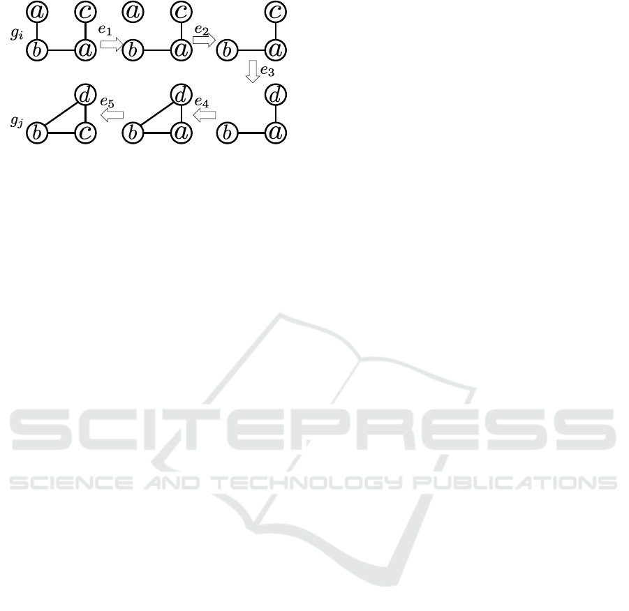
Figure 2: Sequence of edit operations for transforming g
i
into g
j
.
3 PROPOSED GRAPH KERNELS
The definition of d(g
i
,g
j
) is vital for the performance
of the classification model. There are various frame-
works for designing graph kernels. Two representa-
tive frameworks among them are based on graph edit
distance and graph relabeling. First, we propose a
novel graph kernel based on the former framework,
and then we propose another novel graph kernel based
on both frameworks.
3.1 Graph Kernels based on Graph Edit
Distance
Graph edit distance is one of the most representative
metrics for defining d(g
i
,g
j
), and a number of graph
kernels based on the graph edit distance have been
proposed (Neuhaus and Bunke, 2007). The graph edit
distance between graphs g
i
and g
j
is defined as the
minimum length of the sequence of edit operations
needed to transform g
i
into g
j
, where one edit opera-
tion includes the insertion or deletion of a vertex/edge
and substitution of a vertex label. Although edit dis-
tance was originally proposed for measuring the dis-
similarities between two strings, the metric was ex-
tended to graphs because edit operations were intro-
duced for graphs.
Figure 2 shows a certain sequence of edit oper-
ations that consists of one deletion of vertex (e
2
),
one insertion of edge (e
4
), one deletion of edge (e
1
),
and two substitutions of labels (e
3
,e
5
). The compu-
tation needed to obtain the edit distance between g
i
and g
j
is equivalent to searching for the minimum
length of the sequence of edit operations needed to
transform g
i
into g
j
. The method based on the A
⋆
al-
gorithm is a well-known method for computing the
exact graph edit distance (P. Hart, et. al, 1968). How-
ever, this method cannot be applied to graphs of large
size, because the problem of obtaining the exact graph
edit distance between two graphs is known to be NP-
hard and consequently, the graph kernels based on the
graph edit distance have drawback in terms of com-
putational efficiency. To address this drawback, we
propose a graph kernel based on the mapping dis-
tance (Zhiping, et. al, 2009) (Riesen and Bunke,
2009), which is the suboptimal graph edit distance be-
tween graphs.
Here, we explain the mapping distance between
graphs. The distance is one method for approximately
measuring the graph edit distance, and this metric is
obtained in O(υ
3
), where υ = max{|V(g
i
)|,|V(g
j
)|}.
To obtain the mapping distance, we use star structures
in the graph. A star structure s(v) for v in a graph
g is a subtree whose root is v and leaves consist of
N(v). That is, s(v) is equivalent to st(v,1). Given a
graph g, |V(g)| star structures can be generated from
g. The multiset of star structures generated from
g is denoted as S(g) = {s(v
1
),s(v
2
),··· , s(v
|V(g)|
)}.
The star edit distance between s(v
i
) and s(v
j
) is the
minimum length of the sequence of edit operations
needed to transform s(v
i
) into s(v
j
) and is denoted as
λ(s(v
i
),s(v
j
)), where λ(s(v
i
),s(v
j
)) is defined as
λ(s(v
i
),s(v
j
)) = λ
1
(v
i
,v
j
) + λ
2
(N(v
i
),N(v
j
))
+ λ
3
(N(v
i
),N(v
j
)),
where
λ
1
(v
i
,v
j
) = δ(ℓ(v
i
),ℓ(v
j
)),
λ
2
(N(v
i
),N(v
j
)) =
|N(v
i
)| − |N(v
j
)|
, and
λ
3
(N(v
i
),N(v
j
)) = max{|N(v
i
)|,|N(v
j
)|}
−|L(N(v
i
)) ∩ L(N(v
j
))|.
Star edit distance λ
1
(v
i
,v
j
) returns 1 if the roots of the
star structures have identical labels and 0 otherwise,
which is equivalent to a substitution for the labels of
roots. Distance λ
2
(N(v
i
),N(v
j
)) equals the required
number of insertions and/or deletions of edges in s(v
i
)
and s(v
j
). Distance λ
3
(N(v
i
),N(v
j
)) equals the re-
quired number of substitutions for labels of leaves in
s(v
i
) and s(v
j
). From the above, λ(s(v
i
),s(v
j
)) repre-
sents the star edit distance between s(v
i
) and s(v
j
).
Given two multisets of star structures S(g
i
) and
S(g
j
), the mapping distance between g
i
and g
i
is de-
noted as md
1
(g
i
,g
j
) and defined as
md
1
(g
i
,g
j
) = min
P
∑
s(u)∈S(g
i
)
λ(s(u),P(s(u))), (2)
where P : S(g
i
) → S(g
j
) is a bijective function. The
computation of md
1
(g
i
,g
j
) is equal to solving the
minimum weight matching on the complete bipar-
tite graph g
′
= (V
i
,V
j
,E
′
) such that for every two
vertices (v
i
,v
j
) ∈ V
i
× V
j
, there is an edge whose
weight is the star edit distance λ(s(v
i
),s(v
j
)) be-
tween s(v
i
) and s(v
j
). Given a square matrix in
Mapping Distance Graph Kernels using Bipartite Matching
63
ϯ
Ϭ
ϱ
Ϯ
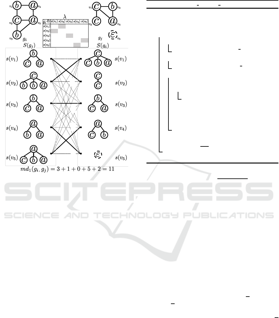
Figure 3: Minimum weight matching to find the mapping
distance between g
i
and g
j
.
which the (i, j)-element represents the star edit dis-
tance λ(s(v
i
),s(v
j
)), this matching problem is solved
by means of the Hungarian algorithm, which runs in
O(υ
3
) (Kuhn, 1955), where υ = max{|V
i
|,|V
j
|}.
Figure 3 shows an example of mapping S(g
i
) to
S(g
j
) to obtain md
1
(g
i
,g
j
). Given two graphs g
i
and
g
j
, five star structures are generated from g
i
and four
star structures are generated from g
j
. The table be-
tween g
i
and g
j
represents the star edit distance be-
tween every pair of star structures in S(g
i
) and S(g
j
).
If |V(g
i
)| does not equal |V(g
j
)|, the matrix that rep-
resents star edit distances among star structures is not
square and cannot be used as an input for the Hungar-
ian algorithm. In order to obtain a square matrix, a
dummy vertex (denoted as v
5
in g
j
) whose label is
ε is inserted in g
j
to equalize the numbers of ver-
tices in g
i
and g
j
. By applying the Hungarian al-
gorithm, the optimal bipartite graph matching (indi-
cated by solid lines) is output and the final answer
md
1
(g
i
,g
j
) = 3+ 1 + 0+ 5+ 2 = 11 is obtained.
Using the mapping distance, we propose a novel
graph kernel called MDKS.
MDKS: We adopt the mapping distance defined in
Eq. (2) to the graph kernel defined in Eq. (1). Given
two graphs g
i
and g
j
, the graph kernel in MDKS is
defined as follows:
Algorithm 1: Mapping Distance Kernel1.
Data: a set of graphs D for training and
variance σ
2
Result: kernel matrix K
1 for g
i
,g
j
∈ D do
2 while |V(g
i
)| < |V(g
j
)| do
3 V(g
i
) ← V(g
i
) ∪ {dummy vertex};
4 while |V(g
i
)| > |V(g
j
)| do
5 V(g
j
) ← V(g
j
) ∪ {dummy vertex};
6 for (v
a
,v
b
) ∈ V(g
i
) ×V(g
j
) do
7 λ ← 0;
8 if ℓ
i
(v
a
) 6= ℓ
j
(v
b
) then
9 λ ← 1;
10 λ ← λ + ||N(v
a
)| − |N(v
b
)||;
11 λ ← λ + max{|N(v
a
)|,|N(v
b
)|} −
|L(N(v
a
)) ∩ L(N(v
b
))| ;
12 T
ab
← λ;
13 md
1
← Hungarian(T);
14 K
ij
← exp
−
md
2
1
2σ
2
;
15 return K;
k
MDKS
(g
i
,g
j
) = exp
−
md
1
(g
i
,g
j
)
2
2σ
2
. (3)
Here, k
MDKS
(g
i
,g
j
) is obtained in O(υ
3
), which is
faster than graph kernels based on the exact graph edit
distance.
Algorithm 1 shows the pseudo-code for comput-
ing an MDKS kernel matrix for a set of graphs D. In
Lines 2 to 5, the numbers of vertices in g
i
and g
j
are
equalized. For each pair of vertices in V(g
i
) ×V(g
j
),
the star edit distance between star structures s(v
a
) and
s(v
b
) is measured and set as the (a, b)-th element in
square matrix T, which is given to the Hungarian al-
gorithm. The Hungarian algorithm returns the map-
ping distance according to the optimal bipartite graph
matching in Line 13. In Line 14, Eq. (3) is computed.
These procedures are repeated for everypair of graphs
in D, and Algorithm 1 finally returns a kernel matrix
for D. This algorithm runs in O(n
2
(υ
3
+
dυ
2
)), where
n, υ, and d are the number of graphs in D, the max-
imum number of vertices in the graphs, and the av-
erage degree of the vertices, respectively. Because
d
is bounded by υ, the computational complexity be-
comes O(n
2
υ
3
).
MDKS has a drawback in terms of graph expres-
siveness. The height of the subtrees between which
we measure the mapping distance is limited, and this
causes a leveling off of the graph expressiveness. It
is desirable to measure the edit distance between high
order subtrees, as the edit distance between trees with
m vertices is computed in O(m
3
) (E. D. Demaine,
ICPRAM 2017 - 6th International Conference on Pattern Recognition Applications and Methods
64
et. al, 2009). However, because the paths from the
root to leaves in a subtree are not simple in the graph
from which the subtree is generated, the number of
vertices in the subtrees increases exponentially for
h, which makes measuring the edit distance between
s(v
i
,h) and s(v
j
,h) intractable. Another way (Carletti,
et. al, 2015) is to use subgraphs of g each of which
consists of vertices within h step from v
i
instead of
star structures of G. However, we require exact dis-
tances between subgraphs of g
i
and subgraphs of g
j
,
which need computation time. In the next subsection,
we propose another efficient graph kernel that com-
pares the characteristics of two subtrees st(v
i
,h) and
st(v
j
,h) for h > 1.
3.2 Graph Kernels based on Relabeling
Given a graph g
(h)
= (V,E,Σ,ℓ
(h)
), all labels of ver-
tices in g
(h)
are updated to obtain another graph
g
(h+1)
= (V,E,Σ
′
,ℓ
(h+1)
). We call the operation a re-
label, and it is defined as ℓ
(h+1)
(v) = r(v, N(v),ℓ
(h)
).
Weisfeiler-Lehman Subtree Kernel (WLSK) (Sher-
vashidze, et. al, 2011), Neighborhood Hash Kernel
(NHK) (Hido and Kashima, 2009), and Hadamard
Code Kernel (HCK) (Kataoka and Inokuchi, 2016)
are representative graph kernels based on this relabel-
ing framework. The vertex label of WLSK is repre-
sented as a string and a relabel for vertex v is defined
as a string concatenation of the labels of N(v). In
NHK, the vertex label is represented as a fixed-length
bit string and relabeling v is defined as logical oper-
ations such as an exclusive-or on the labels of N(v).
The label of HCK is based on the Hadamard code,
which is used in spread spectrum-based communica-
tion technologies, and a relabel for v is defined as a
summation on the labels of N(v).
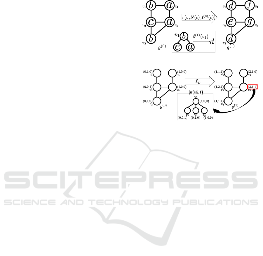
Figure 4 shows an example of the framework
based on graph relabeling. Let g
(0)
be original graph
whose vertices have labels a, b, and c. Each of the
labels is relabeled to obtain g
(1)
. Although the con-
crete calculation depends on the method of relabeling
such as NHK, WLSK, or HCK , it is common that a
relabel for v is applied using v, N(v) and ℓ
(0)
(v). In
the center of Fig. 4, ℓ
(0)
(v
1
) = b is relabeled into d
using adjacent vertices v
2
, v
4
, and its original label
b. Therefore, ℓ
(1)
(v
1
) = d represents the characteris-
tics of st(v
1
,1). The labels of v
1
and v
3
in g
(1)
are
identical labels because st(v
1
,1) = st(v
3
,1) in g
(0)
. It
is desirable to define labels as identical if and only
if both their own labels and labels of adjacent nodes
are also identical. However, realizing this condition
is hard, and it is important to design a relabel method
that satisfies this condition as much as possible.
The label of each vertex is relabeled iteratively.
Figure 4: Example of relabeling (g
(0)
→ g
(1)
).
Figure 5: Example of relabeling in LAK.
Labeling ℓ
(h)
(v), obtained by iteratively relabeling h
times, has a distribution of labels that is reachable
within h steps from v. Therefore, ℓ
(h)
(v) represents
the characteristics of st(v, h). Let {g
(0)
,g
(1)
,··· , g
(h)
}
be a series of graphs obtained by iteratively applying
a relabeling h times, where g
(0)
is an original graph
contained in D. Kernel k(g
i
,g
j
) is defined as
k(g
i
,g
j
) = k(g
(0)
i
,g
(0)
j
) + k(g
(1)
i
,g
(1)
j
)
+··· + k(g
(h)
i
,g
(h)
j
). (4)
The Label Aggregate Kernel (LAK) (Kataoka and
Inokuchi, 2016) is another graph kernel based on this
framework. Next, we present a concrete definition of
a relabel in LAK.
In LAK, ℓ
ℓ
ℓ
(0)
L
(v) is a vector in |Σ|-dimensional
space. If a vertex in a graph has a label σ
i
from the set
Σ = {σ
1
,σ
2
,··· , σ
|Σ|
}, the i-th element in the vector
is 1, and the other elements are 0. In LAK, ℓ
ℓ
ℓ
(h)
L
(v) is
defined as
ℓ
ℓ
ℓ
(h)
L
(v) = ℓ
ℓ
ℓ
(h−1)
L
(v) +
∑
u∈N(v)
ℓ
ℓ
ℓ
(h−1)
L
(u).
The i-th element in ℓ
ℓ
ℓ
(h)
L
(v) equals the frequency of oc-
currence of σ
i
in st(v, h). Therefore, ℓ
ℓ
ℓ
(h)
L
(v) has infor-
mation on the distribution of labels in st(v,h), which
means that ℓ
ℓ
ℓ
(h)
L
(v) is more expressive than the star
structure s(v) used to measure the mapping distance.
We show an example of relabeling in LAK in
Fig. 5, assuming that |Σ| = 3 and relabeling is applied
only once. Consider graph g
(0)
, whose vertices have
labels (1,0,0), (0,1, 0), and (0, 0, 1). We next apply
the relabeling to the graphs to obtain g
(1)
. The label
Mapping Distance Graph Kernels using Bipartite Matching
65
of vertex v in g
(1)
represents the distribution of labels
contained in st(v,1). For instance, the label of v
5
in
g
(1)
is ℓ
ℓ
ℓ
(1)
L
(v
5
) = (2, 1, 1), which indicates that there
are two vertices labeled (1, 0, 0), one vertex labeled
(0,1, 0), and one vertex labeled (0,0,1). This distri-
bution is equivalent to that of the labels contained in
st(v
5
,1). In LAK, the kernel function is defined as
k(g
(h)
i
,g
(h)
j
) =
∑
(v
i
,v
j
)∈V(g
(h)
i
)×V(g
(h)
j
)
δ(ℓ
ℓ
ℓ
(h)
L
(v
i
),ℓ
ℓ
ℓ
(h)
L
(v
j
)).
Using the labels used in LAK, we propose another
novel graph kernel called MDKV.
MDKV: Given two labels ℓ
ℓ
ℓ
(h)
L
(v
i
) and ℓ
ℓ
ℓ
(h)
L
(v
j
), we
denote the distance between ℓ
ℓ
ℓ
(h)
L
(v
i
) and ℓ
ℓ
ℓ
(h)
L
(v
j
) as
τ(ℓ
ℓ
ℓ
(h)
L
(v
i
),ℓ
ℓ
ℓ
(h)
L
(v
j
)), defined as
τ(ℓ
ℓ
ℓ
(h)
L
(v
i
),ℓ
ℓ
ℓ
(h)
L
(v
j
)) = ||ℓ
ℓ
ℓ
(h)
L
(v
i
) − ℓ
ℓ
ℓ
(h)
L
(v
j
))||
2
. (5)
Given two graphs g
(h)
i
and g
(h)
j
relabeled iteratively h
times, the distance between g
(h)
i
and g
(h)
j
is denoted as
md
2
(g
(h)
i
,g
(h)
j
) and defined as
md
2
(g
(h)
i
,g
(h)
j
) = min
Q
∑
u∈V(g
(h)
i
)
τ(ℓ
ℓ
ℓ
(h)
L
(u),ℓ
ℓ
ℓ
(h)
L
(Q(u))),
(6)
where Q : V(g
(h)
i
) → V(g
(h)
j
) is a bijective function.
The computation of md
2
(g
(h)
i
,g
(h)
j
) is also equal to
solving the minimum weight matching on a complete
bipartite graph and is obtained by means of the Hun-
garian algorithm. By combining Eqs. (1), (4), and
md
2
, k
MDKV
(g
i
,g
j
) is defined as follows:
k
MDKV
(g
i
,g
j
) =
h
∑
t=0
k(g
(t)
i
,g
(t)
j
)
=
h
∑
t=0
exp
−
md
2
(g
(t)
i
,g
(t)
j
)
2
2σ
2
The notable difference between MDKS and
MDKV is that while the inputs for md
1
are multisets
of st(v,1), the ones for md
2
are multisets of vectors
obtained from higher order subtrees st(v,h). That is,
the computation of MDKV between two graphs con-
tains larger subgraphs in the two graphs. If we di-
rectly measure the edit distance between s(v
i
,h) and
s(v
j
,h), the number of vertices in s(v,h) exponen-
tially increases when h increases. In this case, MDKV
needs a huge amount of computation time to compute
the edit distance. However, by using a vector repre-
sentation for the vertices and their relabeling, our pro-
posed kernel computes a mapping distance between
s(v
i
,h) and s(v
j
,h) efficiently.
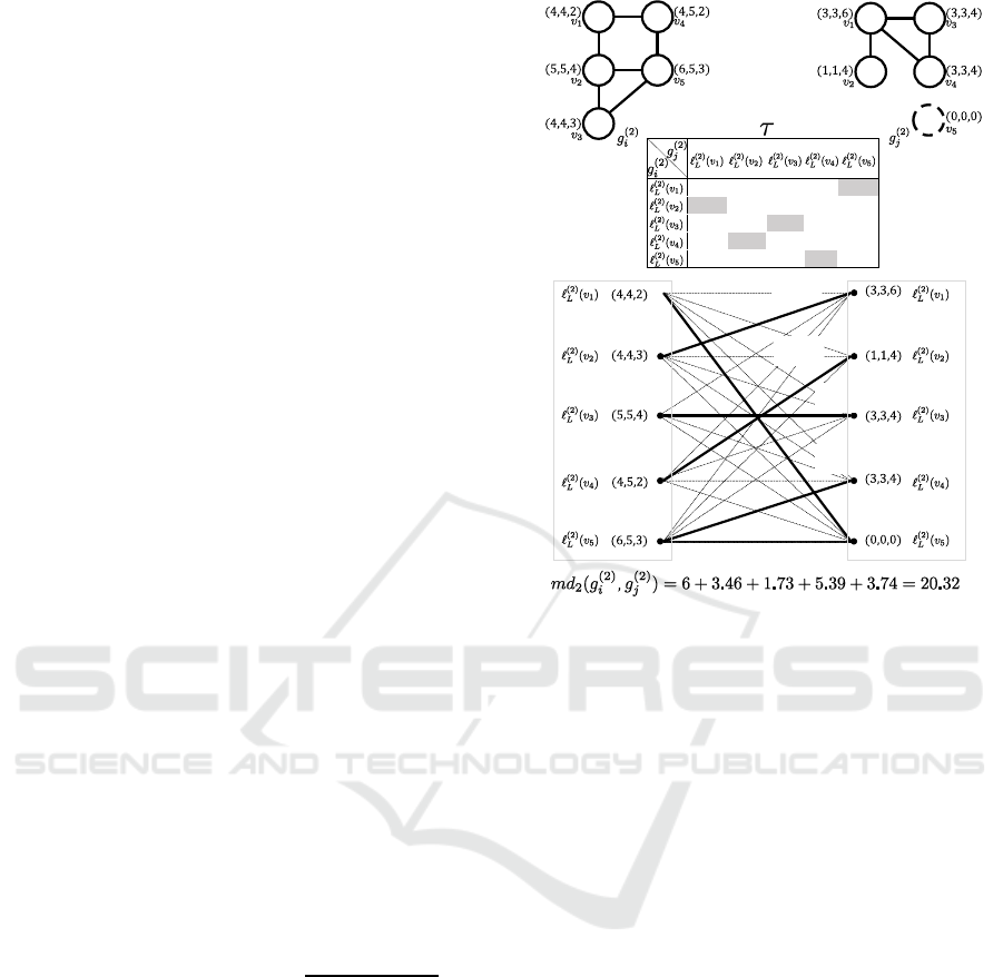
Figure 6: Computation for obtaining md
2
(g
(2)
i
,g
(2)
j
).
Figure 6 shows an example of the procedure to
obtain md
2
(g
(2)
i
,g
(2)
j
), assuming that |Σ| = 3. Graphs
g
(2)
i
and g
(2)
j
are obtained by relabeling given graphs
g
(0)
i
and g
(0)
j
iteratively twice. After relabeling, the
Euclidean distance between every pair of labels in
g
(2)
i
and g
(2)
j
are measured. The table between g
(2)
i
and g
(2)
j
represents the Euclidean distance of every
pair of labels. To equalize the number of vertices in
g
(2)
i
and g
(2)
j
, a dummy vertex whose label is (0, 0,0)
is inserted to g
(2)
j
. The minimum weight matching
is solved by means of the Hungarian algorithm, and
the final answer of md
2
(g
(2)
i
,g
(2)
j
) = 6+3.46+1.73+
5.39+ 3.74 = 20.32 is obtained.
Algorithm 2 shows the pseudo-code for comput-
ing an MDKV kernel matrix for a set of graphs D. In
Lines 5 to 8, the numbers of vertices in g
i
and g
j
are
equalized. For each pair of vertices in V(g
i
) ×V(g
j
),
the Euclidean distance between two vectors ℓ
ℓ
ℓ
(t)
L
(v
a
)
and ℓ
ℓ
ℓ
(t)
L
(v
b
) is measured and set as the (a, b)-th ele-
ment in T. The Hungarian algorithm returns the map-
ping distance according to the optimal bipartite graph
matching in Line 11. Its output using the Gaussian
kernel is added to K
ij
. In Lines 14 to 16, where Z is
a set of non-negative integers, g is relabeled to obtain
g
(t+1)
. These processes in Lines 9 to 15 are repeated
ICPRAM 2017 - 6th International Conference on Pattern Recognition Applications and Methods
66
Algorithm 2: Mapping Distance Kernel2.
Data: a set of graphs D for training and
variance σ
2
Result: kernel matrix K
1 K ← 0;
2 D
(0)
← D;
3 for t ∈ [0, h] do
4 for g
i
,g
j
∈ D
(t)
do
5 while |V(g
i
)| < |V(g
j
)| do
6 V(g
i
) ← V(g
i
) ∪ {dummy vertex};
7 while |V(g
i
)| > |V(g
j
)| do
8 V(g
j
) ← V(g
j
) ∪ {dummy vertex};
9 for (v
a
,v
b
) ∈ V(g
i
) ×V(g
j
) do
10 T
ab
← τ(ℓ
ℓ
ℓ
(t)
L
(v
a
),ℓ
ℓ
ℓ
(t)
L
(v
b
));
11 md
2
← Hungarian(T);
12 K
ij
← K
ij
+ exp
−
md
2
2
2σ
2
;
13 D
(t+1)
←
/
0 ;
14 for g ∈ D
(t+1)
do
15 g
(t+1)
← (V(g), E(g), Z
|Σ|
,ℓ
(t+1)
);
16 D
(t+1)
← D
(t+1)
∪ {g
(t+1)
};
17 return K;
h + 1 times. This algorithm runs in O(h(n
2
υ
3
+
n
2
|Σ|υ
2
+ nd|Σ|υ)), because the computational com-
plexities of Lines 11, 10, and 15 are O(υ
3
), O(|Σ|υ
2
),
and O(
d|Σ|υ), respectively. Because d is bounded by
υ, the computational complexity of Algorithm 2 be-
comes O(hn
2
(υ
3
+ |Σ|υ
2
)).
4 EVALUATION EXPERIMENTS
In this section, we compare the performance of our
graph kernels MDKS and MDKV through numeri-
cal experiments. We implemented the proposed graph
kernels MDKS and MDKV in Java. All experiments
were done on an Intel Xeon E5-2609 2.50 GHz com-
puter with 32 GB memory running Microsoft Win-
dows 7. To learn from the kernel matrices generated
by the above graph kernels, we used the LIBSVM
package
1
using 10-fold cross validation.
4.1 Evaluation using Synthetic Datasets
We examine the computational performance of the
proposed graph kernels by means of synthetic graph
datasets to confirm that the proposed graph kernels
run in O(n
2
(υ
3
+
dυ)) and O(h(n
2
υ
3
+ n
2
|Σ|υ
2
+
1
http://www.csie.ntu.edu.tw/∼cjlin/libsvm/
Table 1: Parameters of the artificial datasets.
Parameters Defaults
Number of graphs in a dataset n =100
Average number of vertices in a graph υ =50
Average degrees of a graph
d =2
Number of distinct labels in a dataset
|Σ| =10
0'.9
0'.6
Figure 7: Computation time for various n.
n
d|Σ|υ)), respectively. We generated graphs with a
set of four parameters . Their default values are listed
in Table 1.
For each dataset, n graphs, each with an average
of
υ vertices, were generated. Two vertices in a graph
were connected with probability
d
υ−1
, and one label
from |Σ| was assigned to each vertex in the graph. The
computation times shown in this subsection are the
average of ten trials.
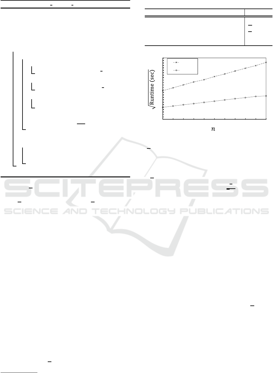
We first varied only n to generate various datasets
in which the other parameters were set to their default
values. The number of graphs in each dataset was
varied from 10 to 100. Figure 7 shows the computa-
tion time needed to generate a kernel matrix for each
dataset for the proposed graph kernels. In this exper-
iment, h was set to 3. As shown in Fig. 7, the square
root of the computation time for the graph kernels is
proportional to the number of graphs in the dataset.
That is, the computation time is proportional to the
square of the number of graphs in the dataset. This
is because the proposed graph kernels are computed
for two graphs, and the kernels runs for all pairs of
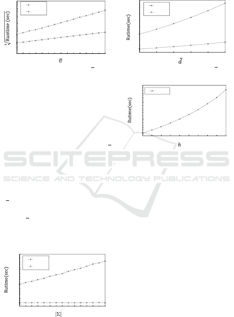
graphs in the dataset. We next varied only
υ to gen-
erate various datasets with the other parameters set
to their default values. Figure 8 shows the computa-
tion time required to generate a kernel matrix in each
dataset when the number of vertices in each dataset
was varied from 50 to 120. The cubic root of the
computation time for the proposed graph kernels is
almost proportional to the average number of vertices
in the datasets. The parts that need a large amount
of computation time in Algorithms 1 and 2 are those
that include the Hungarian algorithm. The computa-
Mapping Distance Graph Kernels using Bipartite Matching
67
0'.9
0'.6
Figure 8: Computation time for various υ.
tion time of the algorithm is proportional to the cube
of the number of vertices of the bipartite graph that
is given as input. In MDKV, τ(ℓ
ℓ
ℓ
(h)
L
(v
i
),ℓ
ℓ
ℓ
(h)
L
(v
j
)) rep-
resents the dissimilarity between s(v
i
,h) and s(v
j
,h).
The number of vertices in s(v,h) exponentially in-
creases as h increases. If we directly measure the edit
distance between s(v
i
,h) and s(v
j
,h), MDKV needs a
huge amount of computation time. However, by using
a vector representation of vertices and the relabeling
for the vertices, our proposed MDKV kernel gener-
ates the kernel matrix efficiently.
In Figs. 9 and 10, we respectively varied |Σ| and
d
to generate various datasets. MDKV needs a compu-
tation time that is proportional to |Σ| in order to com-
pute the Euclidean distance τ(ℓ
ℓ
ℓ
(h)
L
(v
i
),ℓ
ℓ
ℓ
(h)
L
(v
j
)) and
relabel the vertices for the |Σ| dimensional vectors.
The computation times for the propose graph kernels
are almost proportional to the average number of de-
gree of each vertex and the number of vertex labels.
MDKS needs a computation time that is proportional
to d in order to measure the edit distance of the sub-
stitutions for the leaf labels in the star structures. In
contrast, MDKV needs a computationtime that is pro-
portional to
d and |Σ| in order to relabel graphs.
Finally, we varied only h for a dataset generated
with all other parameters set to their default values.
Figure 11 shows the computation time required to
generate a kernel matrix in each dataset when h was
0'.9
0'.6
Figure 9: Computation time for various |Σ|.
0'.9
0'.6
Figure 10: Computation time for various d.
0'.9
Figure 11: Computation time for various h.
varied from 0 to 15. The computation time is propor-
tional to h.
4.2 Classification Accuracy
We compare the classification accuracies of the pro-
posed graph kernels with those of conventional graph
kernels based on the relabeling framework, WLSK,
NHK, and HCK, on three real world datasets, MU-
TAG (Debnath, et. al, 1991), PTC (Helma and
Kramer, 2003), and ENZYMES (Schomburg, et. al,
2004). Since HCK theoretically returns the same val-
ues as LAK returns, classification accuracies of HCK
are equivalent with those of LAK. The first dataset
MUTAG consists of 188 chemical compounds and
their classes are binary values representing whether
each compound is mutagenic. The second dataset
PTC consists of 344 chemical compounds, and their
classes are binary values representing whether each
compound is toxic. Generally, a chemical compound
is represented as a graph with labeled edges, which is
not a graph that is treated in this paper. We treated the
graphs with edge labels in the following two ways: 1)
we ignore the edge labels or 2) an edge labeled ℓ that
is adjacent to vertices u and v in a graph is converted
into a vertex labeled ℓ that is adjacent to u and v, as
explained in (Hido and Kashima, 2009). After con-
ICPRAM 2017 - 6th International Conference on Pattern Recognition Applications and Methods
68
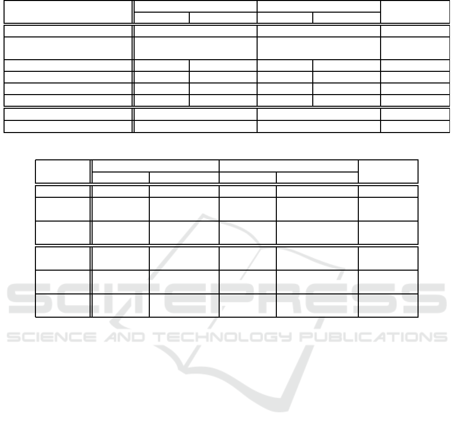
Table 2: Description of evaluation datasets.
MUTAG PTC
ENZYMES
edge labels no edge labels edge labels no edge labels
The number of graphs n 188 344 600
The number of classes 2 2 6
(class distribution) (125,63) (152,192) (100 per class)
Maximum number of vertices 84 40 325 109 126
Average number of vertices 53.9 26.0 77.5 25.6 32.6
Number of labels 12 8 67 19 3
Average Degree 2.1 2.1 2.7 4.0 3.9
σ
min
10 10 10
2
σ
max
10
4
10
5
10
4
Table 3: Classification accuracies.
MUTAG PTC
ENZYMES
edge labels no edge labels edge labels no edge labels
MDKS 92.6% 91.0% 64.2% 63.1% 61.2%
MDKV
94.1% 93.6% 64.0% 66.9% 65.3%
(h = 3) (h = 2) (h = 0) (h = 3) (h = 2)
St-MDKV
91.5% 90.4% 64.9% 64.0% 63.0%
(h = 7, 8) (h = 3) (h = 1, 8) (h = 1) (h = 4)
NHK
92.6% 90.4% 60.8% 55.8% 45.0%
(h = 3, 4) (h = 2) (h = 3, 5) (h = 1, 2,··· ,15) (h = 8)
WLSK
92.0% 90.4% 62.8% 64.2% 58.5%
(h = 3) (h = 1) (h = 15) (h = 10) (h = 1)
HCK
92.0% 91.0% 63.1% 65.4% 57.2%
(h = 3) (h = 1) (h = 15) (h = 12) (h = 4)
verting edges in graphs, labels are assigned to only the
vertices. The third dataset, ENZYMES consists 600
proteins and their classes represent Enzyme Commis-
sion numbers from 1 to 6. Table 2 shows a summary
of each dataset.
Before classifying a dataset that does not contain
graphs but consists of points in a p-dimensional fea-
ture space, we usually normalize the dataset using the
mean µ
q
and standard deviation σ
q
in the q-th feature
(1 ≤ q ≤ p). By normalizing the dataset, we often
obtain an accurate model for classifying the dataset.
Similarly, we apply this procedure in MDKV. To do
so, we use the mean µ
(t)
q
and standard deviation σ
(t)
q
for the |Σ| dimensional vectors to represent the vertex
labels for each t (1 ≤ t ≤ h) and q (1 ≤ q ≤ |Σ|). Us-
ing this procedure, we avoid the exponential increase
in the elements in the vectors representing vertex la-
bels when h is increased. We call the MDKV method
that uses this procedure St-MDKV.
Table 3 shows the classification accuracies of the
proposed and conventional graph kernels . We ex-
amined the highest accuracy for each kernel and each
dataset varying σ of the Gaussian kernel and h. We
varied the σ from σ
min
to σ
max
in intervals of 10 (see
Table 2) and h from 0 to 15 in intervals of 1. As
shown in Table 3, the classification accuracies of the
proposed graph kernels outperform those of the con-
ventional graph kernels. The values of h for MDKV
are relatively low, which indicates that the elements
in the vectors representing vertex labels exponentially
increase and distance τ(ℓ
ℓ
ℓ
(h)
L
(v
i
),ℓ
ℓ
ℓ
(h)
L
(v
j
)) becomes in-
adequate when h increases. However, the values of
h for St-MDKV are high. By normalizing the vec-
tors representing vertex labels, we adequately mea-
sure the (dis)similarity between s(v
i
,h) and s(v
j
,h),
which results in high classification accuracy for vari-
ous datasets.
5 CONCLUSION
In this paper, we proposed two novel and efficient
graph kernels called Mapping Distance Kernel with
Stars (MDKS) and Mapping Distance Kernel with
Vectors (MDKV). MDKS approximately measures
the graph edit distance using star structures of height
one. The method runs in O(υ
3
), where υ is the
maximum number of vertices in the graphs. How-
ever, when the height of the star structures is in-
Mapping Distance Graph Kernels using Bipartite Matching
69

creased to avoid structural information loss, this graph
kernel is no longer efficient. Hence, MDKV repre-
sents star structures of height greater than one as vec-
tors and sums their Euclidean distances. It runs in
O(h(υ
3
+|Σ|υ
2
)), where Σ is a set of vertexlabels and
graphs are iteratively relabeled h times. We verified
the computational efficiency of the proposed graph
kernels on artificially generated datasets. Further, re-
sults on three real-world datasets showedthat the clas-
sification accuracy of the proposed graph kernels is
higher than three conventional graph kernel methods.
REFERENCES
Sch¨olkopf, Bernhard, and Smola, Alexander J.. 2002.
Learning with Kernels. MIT Press.
Kashima, Hisashi, Tsuda, Koji, and Inokuchi, Aki-
hiro. 2003. Marginalized Kernels Between Labeled
Graphs. In Proc. of the International Conference on
Machine Learning (ICML). 321–328.
Zhiping, Zeng, Anthony K.H. Tung, Jianyong Wang, Jian-
hua Feng, and Lizhu Zhou. 2009. Comparing Stars:
On Approximating Graph Edit Distance. In Proc. of
the VLDB (PVLDB). 2(1): 25–36.
Riesen, Kaspar, and Bunkle, Horst. 2009. Approximate
graph edit distance computation by means of bipar-
tite graph matching. Image Vision Computing. 27(7):
950–959.
Hido, Shohei, and Kashima, Hisashi. 2009. A Linear-Time
Graph Kernel. In Proc. of the International Confer-
ence on Data Mining (ICDM). 179–188.
Shervashidze, Nino, Schweitzer, Pascal, Jan van Leeuwen,
Erik, Mehlhorn, Kurt, and Borgwardt, Karsten M..
2011. Weisfeiler-Lehman Graph Kernels. Journal of
Machine Learning Research (JMLR): 2539–2561.
Kataoka, Tetsuya, and Inokuchi, Akihiro. 2016. Hadamard
Code Graph Kernels for Classifying Graphs. In Proc.
of the International Conference on Pattern Recogni-
tion Applications and Methods (ICPRAM). 24–32.
Sch¨olkopf, Bernhard, Tsuda, Koji, and Vert, Jean-Philippe.
2004. Kernel Methods in Computational Biology.
MIT Press.
Kuhn, Harold W.. 1955. The Hungarian Method for the
Assignment Problem. Naval Research Logistics. 2:
83–97.
Bernhard E. Boser, Isabelle, Guyon, and Vladimir, Vapnik.
1992. A Training Algorithm for Optimal Margin Clas-
sifiers. In Proc. of the Conference on Learning Theory
(COLT). 144–152.
Hart, Peter E., Nilsson, Nils J., and Raphael, Bertram. 1968.
A Formal Basis for the Heuristic Determination of
Minimum Cost Paths. Journal of IEEE Trans. Systems
Science and Cybernetics. 4(2): 100–107.
Debnath, Asim Kumar, Lopez de Compadre, Rosa L., Deb-
nath, Gargi, Shusterman, Alan J., and Hansch, Cor-
win. 1991. Structure-Activity Relationship of Mu-
tagenic Aromatic and Heteroaromatic Nitro Com-
pounds. Correlation with Molecular Orbital Energies
and Hydrophobicity. Journal of Medicinal Chemistry
34: 786–797.
Helma, Christoph, and Kramer, Stefan. 2003. A Survey of
the Predictive Toxicology Challenge Bioinformatics
19(10): 1179–1182.
Schomburg, Ida, Chang, Antje, Ebeling, Christian, Gremse,
Marion, Heldt, Christian, Huhn, Gregor, and Schom-
burg, Dietmar. 2004. BRENDA, the Enzyme
Database: Updates and Major New Developments.
Nucleic Acids Research 32D: 431–433.
Chang, Chih-Chung, and Lin, Chih-Jen. 2001. LIBSVM: A
library for support vector machines. Available online
at http://www.csie.ntu.edu.tw/cjlin/libsvm.
Neuhaus, Michel, and Bunke, Horst. 2007. Bridging the
Gap Between Graph Edit Distance and Kernel Ma-
chines. World Scientific.
H. W. Kuhn. 1955. The Hungarian Method for the Assign-
ment Problem. Naval Research Logistics, 2: 83–97.
E. D. Demaine, S. Mozes, B. Rossman, and O. Weimann.
2009. An Optimal Decomposition Algorithm for Tree
Edit Distance. ACM Transaction on Algorithm, 6 (1).
Carletti, Vincenzo, Ga¨uz`ere, Benoit, Brun, Luc, and Vento,
Mario. 2015. Approximate Graph Edit Distance Com-
putation Combining Bipartite Matching and Exact
Neighborhood Substructure Distance. Graph Based
Representations in Pattern Recognition (GbRPR),
188–197.
ICPRAM 2017 - 6th International Conference on Pattern Recognition Applications and Methods
70
