Process Optimization for Cutting Steel-Plates
Markus Rothe, Michael Reyer and Rudolf Mathar
Institute for Theoretical Information Technology, RWTH Aachen University, Kopernikusstraße 16, 52074 Aachen, Germany
Keywords:
Two-Stage Three-Dimensional Guillotine Cutting, Residual Bin-Packing Problem, Mixed Integer Program-
ming Model, Reuseable Leftovers.
Abstract:
In this paper, we consider the two-stage three-dimensional guillotine cutting stock problem with usable left-
over. There are two properties that distinguish our problem formulation from others. First, we allow the items
to be rotated. Second, we consider the case in which leftover material is to be reused in subsequent production
cycles. Third, we solve the problem in three dimensions. The optimization problem is formulated as a mixed
integer linear program. To verify the approach, several examples show that our formulation performs well.
1 INTRODUCTION
In many areas of industrial production large or long
pieces of material need to be cut into smaller ones.
E.g., it needs to be decided from which reel of raw
material a cable of a specific length will be produced.
This is an example for a one-dimensional problem.
An example for a two-dimensional problem is to cut
patterns from pieces of large leather. In our case, we
want to cut items out of slabs of steel. This is a three-
dimensional problem.
The cutting stock problem is similar to the bin
packing problem and the knapsack problem. In the
bin packing problem objects of different sizes must be
packed into a finite number of bins. The classical bin
packing problem minimizes the number of bins that
are used. For the knapsack problem, there is only one
bin of a certain volume and the objects to pack have
a value and a volume. Then, the objective is to maxi-
mize the value of the packed objects. Both problems
are, in general, NP-hard problems.
In this paper, we formulate a problem that is simi-
lar to the above mentioned problems and solves the
cutting stock problem. The problem is formulated
such that the optimization program becomes linear
and we can find an optimal solution according to our
objective function.
The general problem of cutting stock is explored
widely in the literature. The earliest work we found,
that minimizes scrap material, is (Kantorovich, 1960).
We cite the English translation, which is, to the best
of our knowledge, a translation from the original Rus-
sian publication from 1939. (Kurt Eisemann, 1957),
and (Gilmore and Gomory, 1961), utilize linear pro-
gramming to solve cutting stock problems. P. Gilmore
and Gomory investigate the one dimensional prob-
lem of cutting items from stock of several standard
lengths. They devise the method of column gener-
ation in their work. P. Gilmore and Gomory con-
tinued their work in (Gilmore and Gomory, 1965).
Here, they extend their formulation to multistage cut-
ting stock problems of two and more dimensions.
(Farley, 1988), adapt the approach of (Gilmore
and Gomory, 1961), with some practical adaptations.
In particular, they introduce guillotine cuts, which
will be explained in detail in the following section.
Solutions not utilizing linear programming have
also been published, e.g., tree-search algorithms,
(Christofides and Whitlock, 1977). The survey (Hinx-
man, 1980), summarizes many more publications.
(Dyckhoff et al., 1985), give a detailed catalog of cri-
teria for characterization of real-world cutting stock
problems (Dyckhoff et al., 1985). (Yanasse et al.,
1991), describe heuristics for the cutting stock prob-
lem. (Carnieri et al., 1994), formulate the cutting
stock problem as a Knapsack algorithm and also give
heuristics to enhance computational efficiency.
(Kalagnanam et al., 2000), formulate the problem
for the steel industry, without considering the depth
of the slabs. (Martello et al., 2000), present a three-
dimensional bin packing problem, while allowing ar-
bitrary, i.e., non-guillotine, cuts. (Morabito and Are-
nales, 2000), focus on a simplified cutting pattern. In
their book Operations Research: Applications and Al-
gorithms, (Wayne L Winston and Jeffrey B Goldberg,
2004), summarize and extend some of the aforemen-
Rothe M., Reyer M. and Mathar R.
Process Optimization for Cutting Steel-Plates.
DOI: 10.5220/0006108400270037
In Proceedings of the 6th International Conference on Operations Research and Enterprise Systems (ICORES 2017), pages 27-37
ISBN: 978-989-758-218-9
Copyright
c
 2017 by SCITEPRESS – Science and Technology Publications, Lda. All rights reserved
27

tioned as well as many more methods.
(Silva et al., 2010), consider waste, but lack the
third dimension in their problem formulation. They
also mention the value of the surplus material on a
conceptual level, but do not show it in their problem
formulation. (Burke et al., 2011), present an iterative
packing methodology based on squeaky wheel opti-
mization. (Furini and Malaguti, 2013), make similar
formulations as previously found in the literature, but
focus on the run-time of the solution.
The recent results from (Andrade et al., 2013),
lay the foundation for our problem formulation.
(Andrade et al., 2013), investigate two-stage two-
dimensional guillotine cutting stock problems with
usable leftover. We will extend their formulation for
two-stage three-dimensional guillotine cutting stock
problems with usable leftover. The term “stage” will
be explained when we describe the constrains that are
imposed by our production machinery.
There are three properties that distinguish our
problem formulation from others. First, we allow the
items to be rotated.
Second, we consider the case in which leftover
material is to be reused in subsequent production cy-
cles. I.e., after one production cycle, leftover material
is added to the set of slabs.
Third, we solve the problem in three dimensions.
On the one hand, this is needed to calculate the
weight, which is required in our objective function.
On the other hand, this opens up for the possibility to
cut an item from a slab that is thicker than necessary,
if the value of the leftover material permits or even
dictates this decision.
The remainder of the present paper is organized
as follows. In Section 2, we present the problem we
want to solve and the model we use. In Section 3, we
propose an optimization program to solve the prob-
lem. In Section 4, we discuss some examples and
their solutions. Finally, we summarize our results in
Section 5.
2 PROBLEM FORMULATION
AND MODEL DESCRIPTION
The overall goal is to fulfill customer orders of blocks
of steel. We call the ordered blocks of steel items.
These items are cut from larger slabs of steel. As the
size of an item is defined by the customer, the size is,
in general, different and arbitrary from item to item.
The problem we solve in this work is the decision
which item is cut from which slab and how items are
geometrically placed on each slab. Due to the produc-
tion process, or technical and economic restrictions,
(a) (b) (c)
Figure 1: Guillotine cutting in (b) and (c).
these problems can have an abundance of constraints.
It is not important that the material we are working
with is steel. However, the machines that are used
for cutting the slabs create certain constraints in our
problem formulation.
In general, when items are cut from slabs, the orig-
inal slab is cut up into items and surplus material. The
surplus material can either be useful in the future or it
is so small that it is thrown away. If it is kept we call
it leftover material and it will be placed in the set of
slabs for future usage. If it is thrown away we call it
scrap material.
One of our goals is to use surplus material more
frequently than new slabs. Otherwise, the slabs in
stock could increase over time. Our solution for this
problem is to attach a value per kilogram to all the
slabs. The less a slab weights in total, the smaller its
value per kilogram.
The machines cutting the slabs can only do full
straight cuts, parallel to the edges of the slab and not
stop halfway through the material. This is called guil-
lotine cutting.
Figure 1a shows how the blue item can not be cut
from the gray slab if it is placed in the bottom left cor-
ner. The item has either to be cut as seen in Fig. 1b or
Fig. 1c. Leftover material will have different shapes,
not only depending on the exact geometrical place-
ment of the item on the slab, but also depending on the
exact cuts being made. Currently, in order to calculate
the dimensions of the surplus material, the problem
formulation assumes a strict cutting order, which will
be explained shortly.
Our model follows (Lodi and Monaci, 2003), in
using the notion of shelves, as does (Andrade et al.,
2013). Shelves are a way to connect the restriction on
guillotine cutting and geometric placement of items.
Figure 2 shows the general layout of items and shelves
on a slab.
In this figure, item 1 and item 2 are on the same
shelf, while item 3 is on a separate shelf. To make this
clear, a shelf is just a notion to group and place items
on a slab. Further, shelf ν is opened by item ν. The
height of all items, that are placed in this shelf after
item ν must be less than or equal to the height of item
ν. I.e., the height of shelf ν is equivalent to the height
ICORES 2017 - 6th International Conference on Operations Research and Enterprise Systems
28

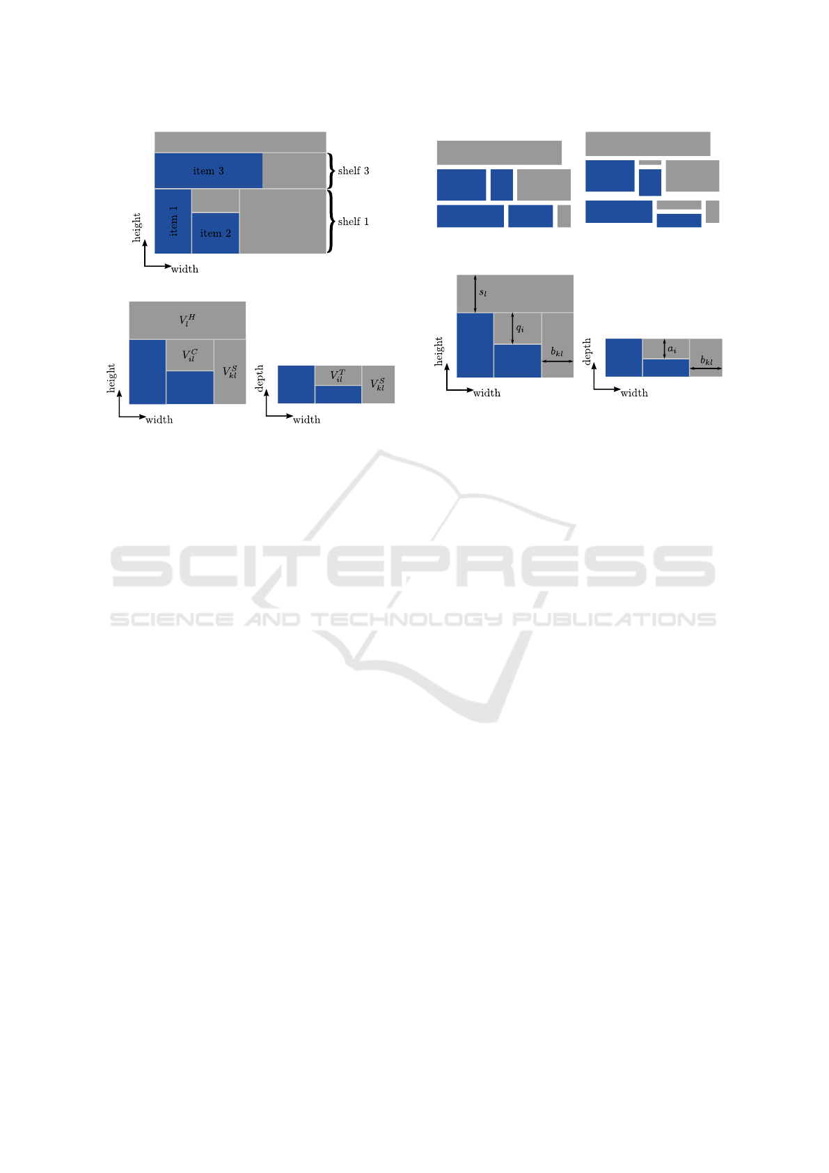
Figure 2: Shelves.
(a) (b)
Figure 3: Positions of leftover material.
of item ν. An item is either placed in an existing shelf
or opens a new shelf. As a result, if item
ˆ
ν was placed
in an existing shelf, then shelf
ˆ
ν does not exist.
As was mentioned earlier, the size and form of
the surplus material depends on the order in which
cuts are made. Therefore, our problem formulation
assumes a specific order of the cuts. This is neces-
sary to calculate the precise dimensions, and hence
the value, of the surplus material. The result of the
cuts is depicted in Fig. 3.
The figure is ambiguous about the depth of V
C
il
,
which is the leftover material filling the height above
item i on slab l. It has the same depth as the slab,
which is clear from the following cutting order.
1. Slabs are cut in the direction of “width” such that
shelves are cut out.
2. Each shelf is cut in the direction of “height” such
that the widths of items are correct.
3. V
C
il
are trimmed from the items.
4. V
T
il
are trimmed from the items.
Trimming in this context means to cut unwanted
pieces from the items, e.g., separating V
T
il
from the
item.
(Andrade et al., 2013), describe their model as
having “two stages”.
In the first stage, parallel longitudinal (hor-
izontal) guillotine cuts are produced on a
plate, without moving it, to produce a set of
strips. In the second stage, these strips are
pushed, one by one, and the remaining parallel
transversal (vertical) guillotine cuts are made
on each strip. ((Andrade et al., 2013, p. 2))
(a) Exact case. (b) Non-exact case.
Figure 4: Two-stage cutting patterns.
(a) (b)
Figure 5: Measuring the leftover material.
Further, (Andrade et al., 2013), distinguish between
the exact and non-exact cases of matching items to
shelves. Figure 4a shows the exact case. Here, all
items in the same shelf have the same height. On the
other hand, Fig. 4b shows the non-exact case. Here,
trimming is necessary, because items in the same shelf
might have a different height. Recall that (Andrade
et al., 2013), only account for two dimensions. They
do not treat trimming as a separate stage.
Our formulation matches items to slabs in three
dimensions considering the non-exact case. Items are
trimmed at most two times, but items are not stacked
in the third dimension. So we call our problem a two-
stage three-dimensional non-exact guillotine cutting
stock problem.
The objective function of our optimization prob-
lem will maximize the value of the surplus material,
accounting for the lost value of cut slabs. A value
needs to be attached to the volumes of the pieces of
surplus material. In order to calculate the volumes,
the measures depicted in Fig. 5 are used.
As we mentioned earlier, the value of each piece
of surplus material is a function of its weight. The
weight of each piece is calculated by simply mul-
tiplying its volume by the weight per volume unit.
The constants g
e
l
define the boundaries of the weight
classes. α
e
l
is the value relative to the value of the slab
the piece originates from. l denoting the slab, e denot-
ing the weight class. Explicit example values for g
e
l
and α
e
l
are given in Table 1. E.g., the value per kilo-
gram of a piece of surplus material weighting between
2.1 kg and 5 kg is 0.5 times the value per kilogram of
the slab it originates from.
Surplus material is considered waste if one of its
sides is too small. See d
W
min
l
, d
H
min
l
, d
T
min
l
in Table 1.
Process Optimization for Cutting Steel-Plates
29

We allow items to be rotated in the width-height-
axis. This is done by copying each item and rotating
the copy. We then restrict placement such that only
one of these items is produced. More on this in the
optimization program itself.
Further, we require items to be sorted by decreas-
ing height, i.e., h
i
≥ h
i+1
. This is a result of how the
height of shelves is determined in our optimization
problem. The first item to be placed in a shelf defines
its height. Only items with a larger index are allowed
to be put into this shelf. So all items following the
first item must have the same or a smaller height, such
that they can be placed on any of the existing shelves.
Therefore, items are sorted by decreasing height be-
fore given an index.
3 THE OPTIMIZATION
PROGRAM
Below is the complete optimization program, which
will be explained afterwards.
Define F
N
= {1, . . . , N} for any N ∈ N. Unless
otherwise mentioned, the constraints apply to ∀i ∈ F
n
,
∀k ∈ F
n
, ∀l ∈ F
p
. n and p are number of items and
number of slabs, respectively, see Table 1.
The main variables are x
ikl
, i.e., it is one if item i
is placed in shelf k on slab l.
maximize
n
∑
i=1
i
∑
k=1
p
∑
l=1
w
i
h
i
t
i
G
l
p
i
x
ikl
(1)
−
p
∑
l=1
M
l
P
l
u
l
(2)
−
p
∑
l=1
(P
0
l
− P
l
)R
l
(3)
+
|V|
∑
j=1
F
j
(4)
subject to all conditions in Table 2 ,
p
∑
l=1
i
∑
k=1
∑
i∈c
i
x
ikl
= 1 ,
∀c
i
= { j | j = i or j is rotated version of i} , (5)
n
∑
k=i+1
p
∑
l=1
x
ikl
= 0 , (6)
u
l
≥
1
n
n
∑
i=1
n
∑
k=1
x
ikl
(7)
b
kl
= W
l
x
kk l
−
n
∑
i=k
w
i
x
ikl
,
∀k ∈ F
n
, ∀l ∈ F
p
, (8)
b
k
=
p
∑
l=1
b
kl
, (9)
s
l
= H
l
u
l
−
n
∑
k=1
h
k
x
kk l
, (10)
q
i
=
p
∑
l=1
i
∑
k=1
(h
k
− h
i
)x
ikl
, (11)
a
i
=
p
∑
l=1
i
∑
k=1
(T
l
−t
i
)x
ikl
, (12)
s
l
≥ d
H
min
l
−
ˆ
H(1 − z
H
l
) , (13)
s
l
≤
ˆ
Hz
H
l
+ d
H
min
l
, (14)
V
H
l
≤ s
l
W
l
T
l
G
l
, (15)
V
H
l
≤ H
l
W
l
T
l
G
l
z
H
l
, (16)
b
k
≥
p
∑
l=1
d
W
min
l
x
kk l
− (1 − z
S
k
)
ˆ
W , (17)
b
k
≤
ˆ
W z
S
k
+
p
∑
l=1
d
W
min
l
x
kk l
, (18)
G
l
V
S
kl
≤ M
l
z
S
k
, (19)
V
S
kl
≤ b
k
h
k
T
l
G
l
, (20)
V
S
kl
≤ W
l
h
k
T
l
G
l
x
kk l
, (21)
q
i
≥
p
∑
l=1
i
∑
k=1
d
H
min
l
x
ikl
− (1 − z
C
i
)
ˆ
H ,
(22)
q
i
≤
ˆ
Hz
C
i
+
p
∑
l=1
i
∑
k=1
d
H
min
l
x
ikl
, (23)
G
l
V
C
il
≤ M
l
z
C
i
, (24)
V
C
il
≤ w
i
q
i
T
l
G
l
, (25)
V
C
il
≤ w
i
H
l
T
l
G
l
i
∑
k=1
x
ikl
, (26)
a
i
≥
p
∑
l=1
i
∑
k=1
d
T
min
l
x
ikl
−
ˆ
T (1 − z
T
i
) ,
(27)
a
i
≤
ˆ
T z
T
i
+
p
∑
l=1
i
∑
k=1
d
T
min
l
x
ikl
, (28)
G
l
V
T
il
≤ M
l
z
T
i
, (29)
V
T
il
≤ w
i
h
i
a
i
G
l
, (30)
V
T
il
≤ w
i
h
i
T
l
G
l
i
∑
k=1
x
ikl
, (31)
R
l
= M
l
−
n
∑
i=1
i
∑
k=1
w
i
h
i
t
i
G
l
x
ikl
| {z }
assigned items
ICORES 2017 - 6th International Conference on Operations Research and Enterprise Systems
30

Table 1: Inputs and Identifiers.
Input or Identifier Description
w
i
, h
i
,t
i
Width, height and depth of item i, with i = 1, . . . , n.
p
i
Value of item i per kilogram.
W
l
, H
l
, T
l
Width, height and depth of slab l, with l = 1, . . . , p.
G
l
Weight per volume unit of slab l, e.g., 7.85 · 10
−6
kg
mm
3
.
M
l
= W
l
H
l
T
l
G
l
Weight of slab l.
ˆ
W = max
l=1,...,p
{W
l
} Greatest width of slabs.
ˆ
T = max
l=1,...,p
{T
l
} Greatest height of slabs.
ˆ
H = max
l=1,...,p
{H
l
} Greatest depth of slabs.
P
0
l
Purchase value of slab l per kilogram.
P
l
Current value of slab l per kilogram.
g
e
l
Boundaries of weight classes, specific to slab l,
e.g.,

g
1
1
g
2
1
g
3
1
g
4
1
= g
m
1

=

0 2.1 5.1 10.1

.
α
e
l
Relative value for weight classes, specific to slab l,
e.g.,

α
1
1
α
2
1
α
3
1
α
4
1
= α
m
1

=

0.2 0.5 0.6 1

.
d
W
min
l
, d
H
min
l
, d
T
min
l
Minimum width, height, and depth before leftover
material is considered waste, e.g., d
W
min
l
= d
H
min
l
= d
T
min
l
= 10 cm
−
n
∑
k=1
V
S
kl
−
n
∑
i=1
V
C
il
−
n
∑
i=1
V
T
il
−V
H
l
, (32)
V :=

V
H
l
> 0 | l = 1, . . . , p

∪

V
S
k
> 0 | k = 1, . . . , n

∪

V
C
i
> 0 | i = 1, . . . , n

∪

V
T
i
> 0 | i = 1, . . . , n

, (33)
z
R
je
g
e
l( j)
≤ V
j
,
∀ j ∈ F
|V|
, ∀e ∈ F
m
, (34)
V
j
< g
e+1
l( j)
+ M
l( j)
(1 − z
R
je
) ,
∀ j ∈ F
|V|
, ∀e ∈ F
m−1
, (35)
m
∑
e=1
z
R
je
= 1 , ∀ j ∈ F
|V|
, (36)
F
je
≤ V
j
P
0
l( j)
α
e
l( j)
,
∀ j ∈ F
|V|
, ∀e ∈ F
m
, (37)
F
je
≤ M
l( j)
P
0
l( j)
α
e
l( j)
z
R
je
,
∀ j ∈ F
|V|
, ∀e ∈ F
m
(38)
In the following, the objective function and the con-
straints will be discussed in detail.
The objective is to maximize the profit from the
production of one batch of items. In general, the profit
is calculated by subtracting the costs from the rev-
enue. The costs, on the one hand, consist of the slabs
that are used for production, see Eq. (2), and the scrap
material, see Eq. (3). The revenue, on the other hand,
consists of the produced items, see Eq. (1), and the
reusable leftover material, see Eq. (4). Note that the
objective function is linear in the variables x
ikl
, u
l
, R
l
,
and F
j
, c.f., Table 2.
From Eq. (5) and Eq. (6) we see that all items have
to be produced. This means Eq. (1) of the objective is
constant and does not influence the optimal solution.
However, we will simplify that for the solver.
If we use a slab, it decreases the revenue. I.e., its
value is subtracted in Eq. (2). The production will re-
sult not only in items that we want to produce. There
will also be surplus material. As discussed earlier this
can either be leftover material or scrap material.
The scrap material originates from a slab with a
purchase value P
0
l
and this is the value we lose if we
throw it away. As we have already accounted for the
current value in Eq. (2), we need to compensate for
that in Eq. (3).
The leftover material is a kind of positive revenue.
It is not being paid for by a customer at this moment,
but it might be in future production cycles. So this
value is added to the objective, and thereby to the rev-
enue, in Eq. (4).
The constraints are described in the following.
Equation (5) describes that each item should only be
produced once. Usage of the set c
i
prevents that both,
the original and the rotated version of an item, are
produced.
Equation (6) means that an item i can only be
placed in shelves 1 to i. In other words, an item can
open a shelf or be placed in an existing one. As items
are sorted by height, this ensures equivalence to the
case where the height of a shelf is not determined by
Process Optimization for Cutting Steel-Plates
31

Table 2: (Auxiliary) Variables.
Variable Description
x
ikl
∈ {0, 1} Set to 1 if item i is placed in shelf k on slab l.
u
l
∈ {0, 1} Set to 1 if slab l is used.
b
kl
≥ 0 Remaining width in shelf k on slab l, see Fig. 5a.
b
k
≥ 0 Remaining width in shelf k, see Eq. (9).
s
l
≥ 0 Remaining height above top shelf on slab l,
see Fig. 5a, Eq. (10).
q
i
≥ 0 Remaining height above item i in its assigned shelf,
see Fig. 5a, Eq. (11).
a
i
≥ 0 Remaining depth above item i in its assigned shelf,
see Fig. 5b, Eq. (12).
V
S
kl
≥ 0 Weight of leftover material filling the width of shelf
k on slab l, see Fig. 3. A shelf is located on exactly one slab, so it is 6= 0
for exactly one combination of k and l or all are 0 if the leftover material
is waste.
V
S
k
=
∑
p
l=1
V
S
kl
≥ 0 Weight V
S
of shelf k.
V
C
il
≥ 0 Weight of leftover material filling the height above
item i on slab l, see Fig. 3. It is 6= 0 for only one combination of i and l
or all equal 0 if waste.
V
C
i
=
∑
p
l=1
V
C
il
≥ 0 Weight V
C
above item i.
V
T
il
≥ 0 Weight of leftover material filling the depth above
item i on slab l, see Fig. 3. It is 6= 0 for only one combination of i and l
or all equal 0 if waste.
V
T
i
=
∑
p
l=1
V
T
il
≥ 0 Weight V
T
above item i.
V
H
l
≥ 0 Weight of leftover material on the top of slab l,
see Fig. 3.
z
S
k
, z
C
i
, z
T
i
, z
H
l
∈ {0, 1} Set to 0 if associated weights are waste.
V
j
≥ 0 , ∀ j ∈ F
|V |
An element from the set V, see Eq. (33).
z
R
je
∈ {0, 1} , ∀ j ∈ F
|V |
Set to 1 if weight j is in class e.
F
je
Value of leftover material j in weight class e.
Not equal 0 for one weight class.
F
j
=
∑
m
e=0
F
je
≥ 0 , The value of weight j.
∀ j ∈ F
|V |
R
l
Weight of leftover material that is waste.
the first, but highest item.
Equation (7) sets u
l
to one if slab l is used.
Equation (8) and Eq. (9) set the variable b
k
which
describes the remaining width in shelf k, see also
Fig. 5. Equation (10), Eq. (11), and Eq. (12) set s
l
,
q
i
, and a
i
, respectively. See also Fig. 5.
Equation (13) and Eq. (14) set the variable z
H
l
to
zero if the associated weight V
H
l
is waste. V
H
l
is con-
sidered waste if s
l
< d
H
min
l
. In that case, z
H
l
in Eq. (14)
can either be 0 or 1, but with Eq. (13) it has to be 0.
Then again, if s
l
≥ d
H
min
l
, z
H
l
in Eq. (13) can either
be 0 or 1, while Eq. (14) sets it to 1.
The weights, which are calculated to get the value
of the leftover material, are best understood by look-
ing at Fig. 3. The weight V
H
l
is calculated in Eq. (15)
and Eq. (16). The latter one is set to zero if it is con-
sidered waste. This is done so that no value is added
for it in the objective function.
In Eq. (17) and Eq. (18) z
S
k
is set to 0 if V
S
kl
is scrap
material. Otherwise, z
S
k
is set to 1. In both equations,
the summation over l “picks” the correct slab as x
kk l
can only be one for one l. Beside of that, it works
analogously to Eq. (13) and Eq. (14).
The next three equations, Eq. (19), Eq. (20), and
Eq. (21), set the weight V
S
kl
. It is set to its actual
value if it is usable, otherwise it is set to 0. To
be more precise, the equations set the upper limit
of the weight and the objective indirectly maximizes
the weight such that the upper limit will be reached.
Equation (19) limits V
S
kl
to the weight of the slab or
sets it to 0 if it is scrap material. Equation (20) and
Eq. (21) need to be interpreted in conjunction. Equa-
ICORES 2017 - 6th International Conference on Operations Research and Enterprise Systems
32

tion (20) limits V
S
kl
as if shelf k is on slab l, which is
not necessarily true. Equation (21) then limits V
S
kl
to 0
if x
kk l
equals 0, i.e., only the correct combination of k
and l lead to a value unequal 0.
Equation (22) and Eq. (23) set z
C
i
in a similar way
as Eq. (17) and Eq. (18) set z
S
k
. The sum to find the
correct d
H
min
l
needs to be a sum over x
ikl
. This is be-
cause an item, not being the first item in a shelf, can
be located on any shelf.
The next three equations, Eq. (24), Eq. (25), and
Eq. (26), set the weight V
C
il
in the same way as
Eq. (19), Eq. (20), and Eq. (21) set V
S
kl
. Equation (26)
has an additional sum, compared to the calculation of
V
S
kl
. The argument here is similar to the one above.
Item i can be located on any shelf, so we sum over the
shelves k in order to pick the correct x
ikl
.
Equation (27) and Eq. (28) set z
T
i
in the same way
as z
C
i
is set. Equation (29), Eq. (30), and Eq. (31)
define the weight V
T
il
in the same way as V
C
il
is defined.
R
l
is the sum of the weight of scrap material from
slab l. It is calculated in Eq. (32) as the remainder
from substracting produced and reusable items from
the slab weight. I.e., everything that is not an item or
reusable leftover is scrap material.
Equation (4) uses the set V , which is defined in
Eq. (33). V is the set of all weights not of size zero.
Recall that these weights are only those that are asso-
ciated to reusable material.
The rest of the constrains are used to finally cal-
culate the value of the reusable material. z
R
je
denotes
if weight j is in the weight class e. Let l( j) denote
the slab on which weight j is located. l( j) is linear,
because V
j
= V
S
k
: l( j) = l ⇔ V
S
kl
> 0, analogously for
C, T. Then, z
R
je
shall equal 1 if g
e
l( j)
≤ V
j
< g
e+1
l( j)
. This
is accomplished by Eq. (34), Eq. (35), and Eq. (36).
Equation (35) will set z
R
je
to zero if V
j
is lighter than
the boundary g
e
. Equation (34) will set z
R
je
to zero if
V
j
is heavier than g
e
. Both these equations allow z
R
je
to be either 0 or 1 if the above inequality holds. In
that case Eq. (36) forces z
R
je
to be 1 and we have our
desired behavior.
With this information we can finally calculate F
je
,
which is the value of V
j
. As the name suggests, it is
non-zero only for one specific value of e. Unfortu-
nately, we cannot multiply V
j
by z
R
je
as we want our
problem to stay linear. Therefore, Eq. (37) sets the up-
per limit of its value regardless of z
R
je
. Then, Eq. (38)
sets an even larger upper limit, but only if z
R
je
equals 1.
Otherwise, it sets it to 0, which is what we want if V
j
does not lie in this specific weight class. In our ob-
jective function, the sum is above F
j
, not F
je
. This is
explained in Table 2.
(a) Our solution.
(b) Solution from (Andrade
et al., 2013).
Figure 6: Example 1, input data No. 1, Table 3.
Table 3: Input data No. 1.
(a) Slabs in stock
ID W H T
1 500 700 45
(b) Items in order
ID w h t
−3 150 400 45
−1 100 300 45
−2 100 300 45
3 400 150 45
1 300 100 45
2 300 100 45
4 EVALUATION
The optimization program was implemented using
CVX, which is an add-on for MATLAB. CVX allows
a high level description of the program, which is close
to the description in Section 3. CVX can use several
solvers. The solver we use is Gurobi ((Gurobi Opti-
mization, Inc., 2016)) as it can solve binary integer
linear programs.
In all examples, the boundaries and relative values
of the weight classes are the ones from Table 1. Also,
the weight per volume is given there.
Please note that some of the slabs had to be drawn
incomplete in order to keep the page size down. This
was done only in areas where no items are placed and
is denoted by a dotted line at the top of the slab.
Example 1
We compare our solution to the one named M
L
1
in
(Andrade et al., 2013), which is also implemented in
CVX/Gurobi. As mentioned earlier, the solution in
(Andrade et al., 2013), solves the problem in two di-
mensions. Therefore, in our example, the thickness of
the ordered items matches the thickness of the slabs in
stock.
Later, we will also show an example where the
thickness between slab and items is different.
Process Optimization for Cutting Steel-Plates
33

Table 4: Input data No. 2.
(a) Slabs in stock
ID W H T
1 350 650 40
2 300 300 40
(b) Items in order
ID w h t
1 200 330 40
2 150 300 40
3 150 300 40
The data from Table 3 produces the solutions
shown in Fig. 6. The table shows the rotated items,
where the item with identifier −i denotes the rotated
version of the item with itentifier i. We will omit these
in later tables. The items in this specific table are also
ordered by height as needed for in our problem for-
mulation.
We denote a cut which should not be necessary in
the final cutting procedure with a dashed line. Our
solution results in two quite large pieces of surplus
material. The solution from (Andrade et al., 2013),
results in a solution with three smaller pieces of sur-
plus material. We also rotated all items before feed-
ing the input to the algorithm from (Andrade et al.,
2013). Still, its solution was to put all three items
side by side, i.e., also creating three pieces of surplus
material. Subjectively, two larger pieces of surplus
material are better than three smaller ones.
Putting the solution from (Andrade et al., 2013)
into our objective function, we get a smaller, i.e.,
worse, objective value. That means, according to our
valuation, we have a better overall value of items and
slabs, compared to the algorithm from (Andrade et al.,
2013). It is also shown that the rotation of items is of
importance.
Example 2
This example, see Fig. 7, underlines how our opti-
mization problem finds really good solutions if slabs
can be filled. There is no leftover material on slab 2,
so slab 1 produces a nice large piece of leftover ma-
terial in addition to a smaller one. The smaller one is
just slightly above the size limitations of scrap mate-
rial, so it is put back to the set of slabs for the next
run, too.
Assume, we rotate item 1 on slab 1. The values
of the used slabs, as well as the value of the produced
items stays the same. Still, the value of the objec-
tive function decreases, because the sum of the values
of the surplus material decreases. Note that, the sum
of the weights of the surplus material stays also the
same. The value of the surplus material decreases,
because the function, described by g
e
l
and α
e
l
, is a
concave function. This function is essential for the
performance of the optimization program.
(a) Slab 1 (b) Slab 2
Figure 7: Example 2, input data No. 2, Table 4.
(a) Input data No. 3 (b) Input data No. 4
Figure 8: Ex. 3, data No. 3 and 4, Tables 5 and 6.
Example 3
Two slightly different variations of input data is exam-
ined in this example. Table 5 shows input data no. 3,
while Table 6 shows input data no. 4. The only differ-
ence is the size in the direction of x of the slab.
Figure 8 shows both solutions. Again, it is all
about the value of the leftover material. It is clear
the solution with the highest value of the leftover ma-
terial is optimal, because all of the items have to be
produced according to the objective function.
With input data No. 4, if the items would be
placed as seen in Fig. 8a, then the value of the leftover
material would be less than is shown. This directly
depends on the weight groups. As a result the weight
groups have to be empirically adjusted, according to
the slab sizes and items ordered.
Table 5: Input data No. 3.
(a) Slabs in stock
ID W H T
1 330 650 40
(b) Items in order
ID w h t
1 200 330 40
2 150 300 40
3 150 300 40
ICORES 2017 - 6th International Conference on Operations Research and Enterprise Systems
34

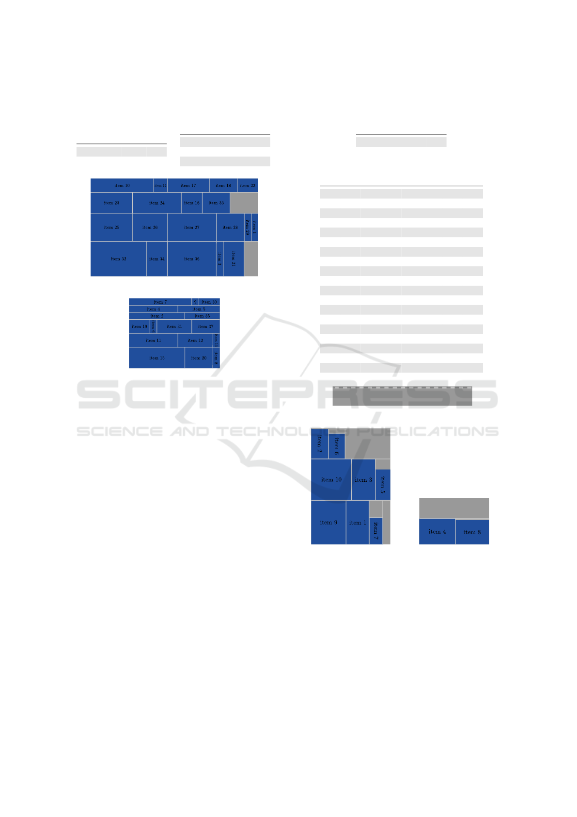
Table 6: Input data No. 4.
(a) Stock
ID W H T
1 350 650 40
(b) Order
ID w h t
1 200 330 40
2 150 300 40
3 150 300 40
(a) Slab 1
(b) Slab 2
Figure 9: Example 4, input data No. 5, Table 7.
Example 4
In Fig. 9 we show the result of an optimization which
barely fits on the slabs and where items have many
similar dimensions. This is where the optimization
problem really shines and a manual solution would
be really time consuming if you would even find one.
Example 5
Compared to the last example, Fig. 10 shows the re-
sult of items, which don’t have many similar sizes.
The result does not look as nice and dense as the pre-
vious one, but it still produces many larger pieces of
surplus material. Note that slab 1 is not used, i.e.,
smaller blocks of steel are used first, because they
have a smaller value. This is exactly what we want.
Example 6
Figure 11 is a slight variation of the previous example.
The sizes of slab 2 and slab 3 are decreased. As a
result not all items fit on these two slabs.
As can be seen from the figure, item 7 is put on
slab 1, but it would neatly fit into the upper right cor-
Table 7: Input data No. 5.
(a) Stock
ID W H T
1 240 140 10
2 130 100 10
(b) Order
ID w h t ID w h t
1 40 10 10 20 40 30 10
2 80 10 10 21 50 30 10
3 50 10 10 22 20 30 10
4 70 10 10 23 60 30 10
5 60 10 10 24 70 30 10
6 20 10 10 25 60 40 10
7 90 10 10 26 50 40 10
8 30 10 10 27 70 40 10
9 10 10 10 28 40 40 10
10 90 20 10 29 10 40 10
11 70 20 10 30 10 30 10
12 50 20 10 31 20 50 10
13 10 20 10 32 80 50 10
14 20 20 10 33 30 40 10
15 80 30 10 34 30 50 10
16 30 30 10 35 10 50 10
17 60 20 10 36 70 50 10
18 40 20 10 37 20 40 10
19 30 20 10
(a) Slab 1
(b) Slab 2 (c) Slab 3
Figure 10: Example 5, input data No. 6, Table 8.
ner of slab 3. The optimization problem can’t find this
solution, because it makes strict assumptions about
the layout of the items. Further investigation about
cutting patterns and their application to the formula-
tion of the optimization problem might be a direction
of future research.
Example 7
In previous examples, the thickness of items matched
Process Optimization for Cutting Steel-Plates
35

Table 8: Input data No. 6.
(a) Stock
ID W H T
1 300 300 45
2 170 250 45
3 150 100 45
(b) Order
ID w h t
1 94 50 45
2 65 37 45
3 51 88 45
4 78 56 45
5 32 66 45
6 54 36 45
7 58 29 45
8 53 72 45
9 95 75 45
10 89 87 45
(a) Slab 1
(b) Slab 2 (c) Slab 3
Figure 11: Example 6, input data No. 7, Table 9.
the thickness of the slabs. Now, we show that our
formulation can give unexpected results if there are
several slabs with different thicknesses to pick from.
In Fig. 12, we show the results of our formulation
with input data no. 8, Table 10. One might assume
that producing the item on slab 2, which matches its
thickness, is the best option. As you can see, our for-
mulation places the item on slab 1, which is consider-
ably thicker than it needs to be. Simply put, the value
Table 9: Input data No. 7.
(a) Stock
ID W H T
1 300 300 45
2 150 220 45
3 120 100 45
(b) Order
ID w h t
1 94 50 45
2 65 37 45
3 51 88 45
4 78 56 45
5 32 66 45
6 54 36 45
7 58 29 45
8 53 72 45
9 95 75 45
10 89 87 45
(a) Slab 1 (b) Slab 2
Figure 12: Example 7, input data No. 8, Table 10.
Table 10: Input data No. 8.
(a) Stock
ID W H T
1 500 700 25
2 500 700 15
(b) Order
ID w h t
1 400 400 15
of the leftover material dictates this placement.
Cuts that trim the thickness can take a long time,
because the area to cut can be quite large compared
to the other cuts. If these trims were not desired, the
optimization problem could either be extended by a
penalty for these cuts or items and orders could sim-
ply be matched in thickness before given to the opti-
mization program.
Runtime and Quality
Besides example 4, the runtime of our examples was
always below one minute, which is a reasonable run-
time to collect and place orders. Example 4 took
about 5000 seconds, which is considerable more than
the other solutions. Limiting the time allowed by the
solver for Example 4 to 60 seconds, we still got a fea-
sible solution. I.e., while not as dense as the solution
shown in Fig. 9, all items were placed on the slabs.
5 SUMMARY
In this paper, we developed an optimization program
that solves the problem of cutting steel-plates, where
only guillotine cuts are allowed. We consider surplus
material as a form of value. Our solution is mod-
eled in three dimensions in order to assign a value
to the surplus material. We use the notion of shelves
to model the placement of items on slabs and allow
items to be rotated.
As has been shown in the examples, our problem
formulation gives subjectively good results, i.e., the
problem is apparently well solved. We have shown
that preferable few, big leftovers are created and small
slabs are used first, see Examples 1 and 6 respectively.
ICORES 2017 - 6th International Conference on Operations Research and Enterprise Systems
36

Example 4 showed that our formulation allows
the tradeoff between runtime and quality. Example 5
showed good performance, even for items of random
size.
In some cases, the placement using shelves might
not be optimal and a more advanced placement might
yield better results in the case of sparser placements.
Consider Example 6, item 7 could fit on slab 3 with
a proper cutting order. Although, modeling and find-
ing optimal solutions of placements not following the
notion of shelves is much more difficult.
Including the third dimension is necessary to
achieve optimal solutions, see Example 7. Our results
are strongly dependent on the choice of weight classes
and their values, see Examples 2 and 3. A proper opti-
mization of these could be the topic of future research.
Although, the values from Table 1 produce good re-
sults for the sizes we used in our examples.
In the future, the number of cuts or a penalty for
using many different slabs could be incorporated eas-
ily into the objective function. But these considera-
tions should be justified by concrete requirements of
a factory.
REFERENCES
Andrade, R., Birgin, E., and Morabito, R. (2013). Two-
stage two-dimensional guillotine cutting stock prob-
lems with usable leftover.
Burke, E. K., Hyde, M. R., and Kendall, G. (2011). A
squeaky wheel optimisation methodology for two-
dimensional strip packing. Computers & Operations
Research, 38(7):1035–1044.
Carnieri, C., Mendoza, G. A., and Gavinho, L. G. (1994).
Solution procedures for cutting lumber into furniture
parts. European Journal of Operational Research,
73(3):495–501.
Christofides, N. and Whitlock, C. (1977). An Algorithm
for Two-Dimensional Cutting Problems. Operations
Research, 25(1):30–44.
Dyckhoff, H., Kruse, H.-J., Abel, D., and Gal, T. (1985).
Trim loss and related problems. Omega, 13(1):59–72.
Farley, A. A. (1988). Practical adaptations of the
Gilmore-Gomory approach to cutting stock problems.
Operations-Research-Spektrum, 10(2):113–123.
Furini, F. and Malaguti, E. (2013). Models for the two-
dimensional two-stage cutting stock problem with
multiple stock size. Computers & Operations Re-
search, 40(8):1953–1962.
Gilmore, P. and Gomory, R. (1961). A Linear Programming
Approach to the Cutting-Stock Problem. Operations
Research, 9(6):849–859.
Gilmore, P. C. and Gomory, R. E. (1965). Multistage Cut-
ting Stock Problems of Two and More Dimensions.
Operations Research, 13(1):94–120.
Gurobi Optimization, Inc. (2016). Gurobi Optimizer Refer-
ence Manual. http://www.gurobi.com/.
Hinxman, A. I. (1980). The trim-loss and assortment prob-
lems: A survey. European Journal of Operational Re-
search, 5(1):8–18.
Kalagnanam, J. R., Dawande, M. W., Trumbo, M., and
Ho Soo Lee (2000). The Surplus Inventory Match-
ing Problem in the Process Industry. Operations Re-
search, 48(4):505–516.
Kantorovich, L. V. (1960). Mathematical Methods of Or-
ganizing and Planning Production. Management Sci-
ence, 6(4):366–422.
Kurt Eisemann (1957). The Trim Problem. Management
Science, 3(3):279–284.
Lodi, A. and Monaci, M. (2003). Integer linear program-
ming models for 2-staged two-dimensional Knapsack
problems. Mathematical Programming, 94:257–278.
Martello, S., Pisinger, D., and Vigo, D. (2000). The Three-
Dimensional Bin Packing Problem. Operations Re-
search, 48(2):256–267.
Morabito, R. and Arenales, M. (2000). Optimizing the cut-
ting of stock plates in a furniture company. Interna-
tional Journal of Production Research, 38(12):2725–
2742.
Silva, E., Alvelos, F., and Valério de Carvalho, J. M. (2010).
An integer programming model for two- and three-
stage two-dimensional cutting stock problems. Euro-
pean Journal of Operational Research, 205(3):699–
708.
Wayne L Winston and Jeffrey B Goldberg (2004). Op-
erations Research: Applications and Algorithms.
Duxbury press Belmont, CA.
Yanasse, H. H., Zinober, A. S. I., and Harris, R. G. (1991).
Two-dimensional Cutting Stock with Multiple Stock
Sizes. Journal of the Operational Research Society,
42(8):673–683.
Process Optimization for Cutting Steel-Plates
37