
Preliminary Evaluation of Symbolic Regression Methods for Energy
Consumption Modelling
R. Rueda, M. P. Cu´ellar, M. Delgado and M. C. Pegalajar
Department of Computer Science and Artificial Intelligence, University of Granada, Granada, Spain
ramon92@correo.ugr.es, manupc@decsai.ugr.es, mdelgado@ugr.es, mcarmen@decsai.ugr.es
Keywords:
Energy Efficiency, Genetic Programming, Straight Line Programs, Pattern Recognition.
Abstract:
In the last few years, energy efficiency has become a research field of high interest for governments and
industry. In order to understand consumption data and provide useful information for high-level decision
making processes in energy efficiency, there is the problem of information modelling and knowledge discovery
coming from a set of energy consumption sensors. This paper focuses in this problem, and explores the use
of symbolic regression techniques able to find out patterns in data that can be used to extract an analytical
formula that explains the behaviour of energy consumption in a set of public buildings. More specifically, we
test the feasibility of different representations such as trees and straight line programs for the implementation of
genetic programming algorithms, to find out if a building consumption data can be suitably explained from the
energy consumption data from other similar buildings. Our experimental study suggests that the Straight Line
Programs representation may overcome the limitations of traditional tree-based representations and provides
accurate patterns of energy consumption models.
1 INTRODUCTION
The implementation of mechanisms to reduce energy
consumption is one of the main objetives at national,
european and international levels (Maros et al., 2016).
In fact, in (Yu et al., 2010) it is shown that energy con-
sumption in Europe and North America had and in-
crease of 1.5% and 1.9% per year (respectively) from
1994 to 2004. Therefore, one of the most important
requirements to address the improvement of energy
efficiency is to perform an effective monitoring of
buildings using sensors, and to use this information
for high-level decision-making processes.
There is a plethora of research proposals in the
literature for extracting knowledge from the sensed
data. Due to paper length limitations, we cannot af-
ford to make an extended revision of the state-of-the-
art in this topic, so we refer the reader to the survey
in (Pan et al., 2014) for a complete review. However,
we emphasize that most of these efforts in knowledge
discovery for energy consumption data might be clas-
sified in two main topics: Energy demand prediction
(Molina-Solana et al., 2014) and creating user profiles
to classify the consumption (Molina-Solana, 2014).
However, in order to perform a more accurate high-
level decision-making processes, it is also necessary
to understand the data using abstraction models, find
hidden relationships in the consumption data, and ex-
tract knowledge useful for the decision making.
In this paper, we address the problem of energy
consumption data modelling and knowledge discov-
ery. More specifically, we test the feasibility of the
use of symbolic regression and genetic programming
to infer an analytical formula that explains the rela-
tionship between the energy consumption data of sim-
ilar buildings in a compound, to analyze and discover
hidden knowledge in energy consumption data. Our
experiments are targeted at testing of different repre-
sentations of algebraic expressions, to know the com-
putational power of each model in practice for the
specific problem of energy consumption modelling.
For that purpose, we select a simple problem in a
real dataset, where a general counter value should be
modelled as aggregation of the energy consumption
data from other 5 different buildings. In the experi-
ments, we show the computational power of two al-
gebraic formula representation mechanisms to infer
the previous relationship, and also the capability of
the learning stage to distinguish between relevant and
non-relevant data for the general counter modelling.
This paper is organized as follows: Section 2 de-
scribes the fundamentals of symbolic regression. Sec-
tions 3 and 4 introduce the representations used in this
research and the genetic operators for each represen-
Rueda, R., Cuéllar, M., Delgado, M. and Pegalajar, M.
Preliminary Evaluation of Symbolic Regression Methods for Energy Consumption Modelling.
DOI: 10.5220/0006108100390049
In Proceedings of the 6th International Conference on Pattern Recognition Applications and Methods (ICPRAM 2017), pages 39-49
ISBN: 978-989-758-222-6
Copyright
c
2017 by SCITEPRESS – Science and Technology Publications, Lda. All rights reserved
39

tation, respectively. Section 5 show the experimenta-
tion of the proporsals over a set of benchmark func-
tions and a real energy consumption dataset. Finally,
conclusions and future research are discussed in sec-
tion 6.
2 FUNDAMENTALS OF
SYMBOLIC REGRESSION
Regression analysis (M., 2007) is one of the basic
tools of scientific research. It is used to fit a func-
tional model that represents a relationship between
independent and dependent variables. Traditionally,
this kind of problems has been solved with algebraic
methods, where the researcher provides a hypothesis
about a functional model with a set of parameters, and
the goal is to optimize these parameters for the studied
dataset. Equation 1 shows the parametric model of re-
gression analysis, where ¯x = (x
1
,x
2
,...,x
n
) stands for
the set of independent variables of the data, f is the
functional model hypothesis, ¯w = (w
1
,w
2
,...,w
m
) are
the parameters of the model, and ¯y = (y
1
,y
2
,...,y
l
)
and the dependent variables of the problem. In these
cases, since ¯x and ¯y are the problem data, and f is a
function established as model hypothesis, the regres-
sion problem is solved by finding the best values for
the parameters ¯w, which are not known in advance.
As an example, the most simple case in regression
analysis is the well known linear regression, whose
functional model can be written as y = f(< w
1
,w
2
>
,x) = w
1
∗ x+ w
2
.
(1)y = f( ¯w, ¯x)
A limitation of classical regression arises when
the data properties are unknown in advance, it is dif-
ficult to find a pattern that explains the dataset, and
therefore it is hard to establish a suitable hypothesis
for the function f. This problem is even less tractable
in the multivariate case, where graphical analyses lack
of enough expresiveness to show relations between
multidimensional data.
To solve these limitations, the use of symbolic re-
gression attempts to generalize the traditional prob-
lem of regression analysis by assuming that f is un-
known, and developing techniques targeted at finding
a suitable model
˜
f and parameters ¯w that minimizes
an error expression such as || ¯y −
˜
f( ¯w, ¯x)||. In sym-
bolic regression it is assumed that ¯y and ¯x and the only
components known in advance. Therefore, the goal of
symbolic regression is to find an algebraic expression
that models the behaviour of the dependent data as
function of independent data. Techniques like genetic
programming (Langdon, 1998) have been developed
to solve this problem.
Symbolic regression techniques have been applied
traditionally in a wide variety of real applications. Be-
sides of being used to solve mathematical optimiza-
tion problems, they have been of practical application
in decision making in economics, chemical processes
optimization, etc. For instance, in (Duffy and Engle-
Warnick, 2002) it is described how can be used sym-
bolic regression to uncover simple data generating
function that have the flavor of strategic rules in eco-
nomic decisions. In the work (McKay et al., 1997),
symbolic regression has been used to model chemical
procesess systems, to solve problems about vacuumm
distillation column and a chemical reactor system. On
the other hand, in (Schmidt and Lipson, 2010) they
explore the use of symbolic regression to perform un-
supervised learning by searching for implicit relation-
ships, specifically they present a successful method
based on implicit derivated. In (Davidson et al., 2001)
the authors use symbolic regression in two real-world
problems, approximating the Colebrook-White equa-
tion and rainfall-runoff modelling.
In this work, we test the feasibility of the use of
symbolic regression to model energy consumption in
a set of public buildings, under the hypothesis that the
resulting models obtained from the symbolic regres-
sion approach will be useful for high-level decision
making processes regarding energy efficiency. The
following subsection describes in depth the basis of
our approach, which is based in genetic programming.
2.1 Introduction to Genetic
Programming
Genetic programming (Langdon, 1998) can be seen
as a supervised learning method based on biological
evolution. Genetic programmingfundamentalsare in-
spired in genetic algorithms, and it has been used in
previous works to solve optimization problems like
symbolic regression (Alonso et al., 2009), digital sig-
nal processing (Alcazar and Sharman, 1996), solving
differential equations (Tsoulos and Lagaris, 2006),
tasks of evolving robotic behaviours (Lazarus and Hu,
2001), grammatical inference (Lankhorst, 1994), au-
tomatic program generation (Koza, 1994), etc. If we
focus in the problem of symbolic regression, the goal
of genetic programming to evolve a set of algebraic
expressions encoded as chromosomes, according to
Darwinian evolution principles of genetic algorithms
and, as fitness measure, the minimization of an er-
ror function that explains the behaviour of dependent
variables regardingthe independentvariables in a spe-
cific dataset.
ICPRAM 2017 - 6th International Conference on Pattern Recognition Applications and Methods
40
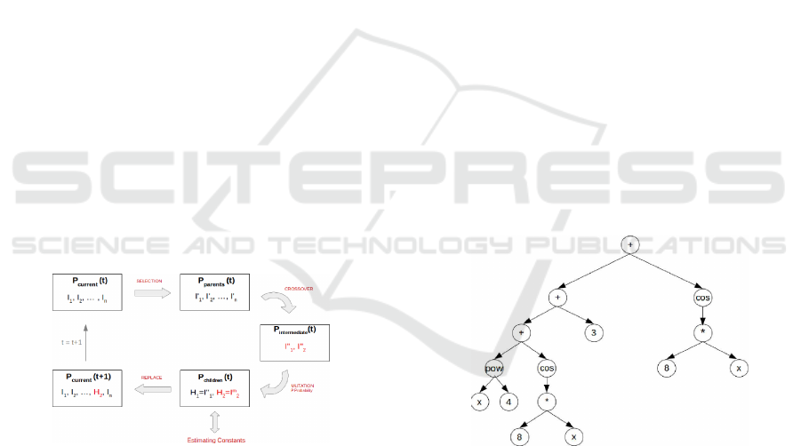
Since the basic structure of genetic programming
is similar to genetic algorithm, figure 1 shows the evo-
lutionary process. Firstly, is generated a set of indi-
viduals, where each individual represents an algebraic
expression. Then, a selection operator is applied to
obtain a subset of individuals or parents which will be
used for genetic recombination. In this work, we use
the tournament selection operator (Pandey, 2016). In
generational evolutionary scheme, there are selected
as parents as many individuals as the size the size
of the initial population. On the other hand, in sta-
tionary scheme, we select just 2 parents. After that,
the crossover operator is applied to generate as many
children individuals as parents. In this work, two par-
ents are recombined to obtain two new children solu-
tions. These children preserve genetic material from
both parents. After the crossover, a mutation oper-
ator takes place over the children with a probability,
imitating biological evolution. Once the previous ge-
netic cycle is finished, the new children are evaluated
according to a fitness measure. In the case of sym-
bolic regression, since it is also neessary to optimize
the function parameters ¯w, in this work, we use the
Simplex method (K. and K., 1989) to obtain an ap-
proximation of ¯w, before the algebraic expressions
encoded into the children are evaluated. Finally, the
initial population is replaced with the new children
and an evolutionary generation is finished. In a gen-
erational scheme, all children replace the whole pop-
ulation, while in the stationary scheme the children
replace their parents.
Figure 1: Genetic Programming Process.
In addition to this basic evolutionary scheme, we
also use an elitism factor, to ensure that the best solu-
tion found during the evolution remains in the popula-
tion. In case that the replacement does not include the
best solution in the new population, this one replaces
the worst solution in it.
Traditionally, each individual is encoded using a
tree structure to represent an algebraic expression in
genetic programming. A new alternativeto encode al-
gebraic expressions is straight line programs (Alonso
et al., 2009) (SLP). A SLP is a lineal structure that
represents a non-linear structure as a graph. This
alternative allows the SLP representation to reuse
subexpressions and represent an algebraic formula in
a structure smaller than trees. So, the main advantages
of SLP representation against tree representation is
the possibility to better explore the search space, be-
ing smaller representations of the same formulas in
SLPs than in trees. In this paper, we make an ex-
perimental evaluation of both approaches to solve our
problem. Both representations are described in the
next section.
3 GENETIC PROGRAMMING
REPRESENTATIONS FOR
SYMBOLIC REGRESSION
3.1 Tree Representation
The traditional representation to encode algebraic ex-
pressions are tree structures (McKay et al., 1995).
This representation allows to generate regular gram-
mars and context-free grammars. On the other hand,
this kind of representations could be limited because
they are non-linear structures represented by non-
linear representations. Thus, the search space is com-
plex, and recombination and mutation operators pro-
posed in the literature may not provide suitable re-
sults.
Figure 2: Example of tree structure.
As an example, one limitation is that tree struc-
tures cannot reuse algebraic subexpressions. In fig-
ure 2 we can see a tree representation of the alge-
braic expression x
4
+ cos(8∗ x) + 3 + cos(8 ∗ x). We
emphasize how we use the expression of cos(8 ∗ x)
in two parts of the tree. Finding such structure with
replicated submodules requires a larger exploration of
the search space, therefore increasing the computing
time in the genetic programming algorithm. In the
same way, a new problem to solve symbolic regres-
sion problems with genetic programming appears, it
is called like bloat (Naoki et al., 2009). This prob-
Preliminary Evaluation of Symbolic Regression Methods for Energy Consumption Modelling
41
lem involves the increased size of analytical formula
obtained by genetic programming, producing unbal-
anced trees with high depth in one branch and low
depth in the other. This fact also makes difficult to
find an optimal solution, and the computing time of
the algorithm is also increased. In order to minimize
the computational complexity, a new representation
called Straight Line Programs is studied in this paper.
3.2 Straight Line Programs
Straight Line Programs are based on Straight Line
Grammars (Benz and K¨otzing, 2013). A Straight
Line Grammar is a non recursive context-free gram-
mar. Straight Line Programs have been used in the lit-
erature to represent algebraic operations (Berkowitz,
1984), geometry problems (Giusti et al., 1998), solv-
ing polynomial equations (Krick, 2002), document
clustering (Sequera et al., 2012), fast sparse matrix-
vector multiplication (Neves and Araujo, 2015) etc.
In the previous section we discussed limitations of
the tree representation. Using Straight Line Programs
as individuals representation in genetic programming,
we pursue to improve our results obtained with tradi-
tional representations like trees. As a consequence,
in our experimentation we show that SLPs represen-
tation implies a minimization of the search space and
computational time against representation.
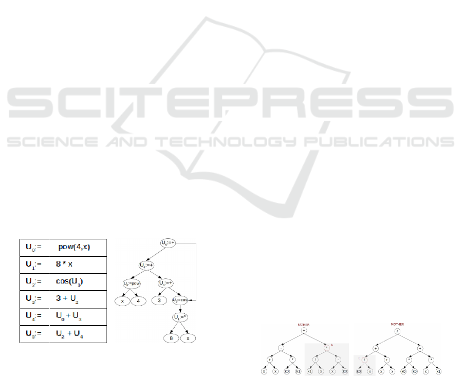
The Straight Line Program structure is represented
by a table. Each row of the table contains an expres-
sion, this expression is built by applying a mathemat-
ical operator (+,-,*,sin, etc...) to a set of operands.
These operands could be variables, constants or ref-
erences to other rows of the table. Figure 3 shows
an example of SLP structure and its graph represen-
tation. To evaluate this algebraic expression we must
evaluate from last element of the table to the begin-
ning.
Figure 3: SLP representation.
Figure 3 shows the advantages of this representa-
tion. It is a linear structure that models a nonlinear
graph structure. Also, this representation allows the
reuse of some algebraic subexpressions in the SLP.
For example, we use cos(8 ∗ x) in two parts of this
representation. Using this structure as representation
of each individual in genetic programming, we reduce
the search space in respect to the tree representation,
and therefore the computing time of genetic program-
ming procedure is also lessen.
4 GENETIC OPERATORS
4.1 Genetic Operators for Tree
Representation
In this section we describe the different crossover and
mutation operators that we use in genetic program-
ming with a tree representation.We assume that the
user has configured a set O = {o
1
,o
2
,...,o
n
} of atomic
operators (+,-,*,sin,cos,...), and T = {t
1
,t
2
,...,t
m
} a
set of terminal symbols. These terminal symbols
encompass the set of independent variables of the
dataset and a set of unknownconstants or function pa-
rameters ¯w. In addition it is required a parameter M
that contains the maximum tree depth allowed. Then,
the individuals in the initial population are generated
as follows:
Firstly, for each individual, it is selected a ran-
dom value l between 2 and M, the current individual
tree depth. Then, it is created the root node contain-
ing an operator selected randomly. The left and right
branches of the operator are also generated randomly
with symbols from the operator set O until level l.
Then, the symbols for these leaf nodes are generated
randomly from the set T. Using this strategy, we
ensure that the initial population contains balanced
trees. After all individuals have been generated with
this procedure, the evolutionary process begins.
4.1.1 Crossover Operator
The aim of this operator is to genetically recombine
two parents to generate two new children. Figure 4
shows two candidates (father on the left, mother on
the right) to generate their corresponding children.
The procedure of this operator is as follows:
Figure 4: Example parent trees for crossover.
A node in the tree is selected at random for each
parent. In the example of figure 4, the selected nodes
ICPRAM 2017 - 6th International Conference on Pattern Recognition Applications and Methods
42
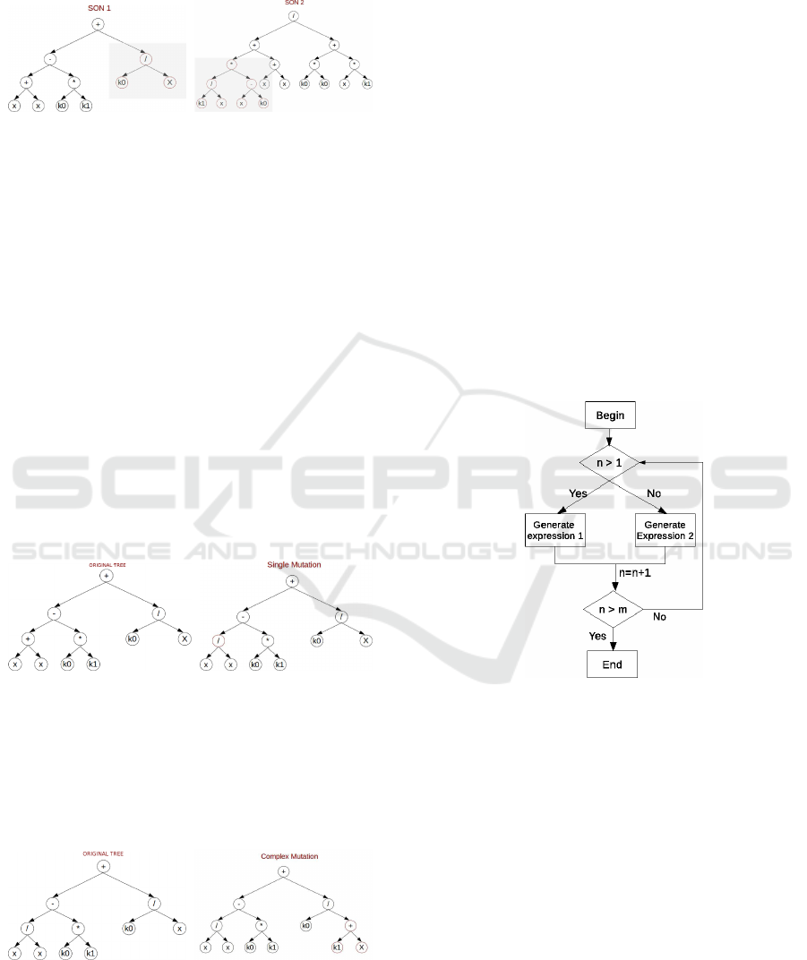
are named as k and t. Then, the two children are gen-
erated by exchanging the subtrees with root k and t in
both parents. This result is shown in figure 5.
Figure 5: Example children trees for crossover.
4.1.2 Mutation Operator
The purpose of this operator is to imitate the be-
haviour of biological evolution, mutating individuals
randomly to improve the exploration of the search
space.
In this representation we use two different muta-
tion operators: One simple whose aim is to main an
explotation of the search space, and other one com-
plex to increase the exploration.
Firstly, figure 6 shows an example of the use of
the simple mutation operator. The simple mutation
operator selects a random node of the tree; then, if
the selected node is a mathematical operator, it is
exchanged for another random operator in O. On
the other hand, if the selected node is a constant or
variable, it is exchanged for another random terminal
symbol in T. Please note that the tree structure is not
altered using this mutation operator.
Figure 6: Example of Simple Mutation Operator.
On the other hand, figure 7 shows the complex
mutation operator. This operator selects a node of the
tree at random, and then this node is pruned and re-
placed with a new randomly generated subtree. As
opposite to the simple mutation operator, the complex
one alters the tree structure of the individual.
Figure 7: Example of Complex Mutation Operator.
In each generation of our genetic algorithm, if a
mutation must be carried out over an individual, it is
selected simple or complex mutation for its applica-
tion with 50% of probability.
4.2 Genetic Operators for SLP
Representation
In this section, we describe the evolutionary opera-
tors for SLPs. To build the initial population, let O =
o
1
,o
2
,...,o
n
be a set of operators (+,-,*,sin,cos,...),
and T = t
1
,t
2
,...,t
m
be a set of terminals. To build
the initial population, figure 8 shows the procedure to
build a new individual containing an algebraic expres-
sion with SLP representation, where n is the number
of rows generated in the SLP during the procedure,
and m is the total size of the SLP table. Also, gener-
ate expression 1 generates a random operator and two
random operands. These operands could be elements
of the set T. On the other hand, generate expression
2 also generates a random operator and two random
operands but, in this case, these operands may be a
symbol in T or a call to previous entries of the SLP
table representation in the range {1..n− 1} .
Figure 8: SLP table creation procedure.
For this representation, new crossover and muta-
tion operators have been developed in (Alonso et al.,
2009). Since these are the only operators we have
found in the literature for SLPs, we will use them
in our experimental evaluation. Future work will be
targeted at developing new crossover and mutation
strategies as part of our research.
4.2.1 Crossover Operator
This section shows the crossover operator applied to
the straight line program representation. This oper-
ator is applied over two individuals or parents. The
procedure of this crossover operator is as follows: A
random position k and t are selected randomly in the
parents’ SLP table. After that, The selected rows and
Preliminary Evaluation of Symbolic Regression Methods for Energy Consumption Modelling
43
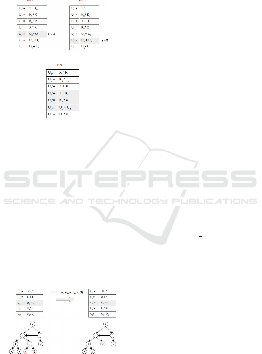
Figure 9: Example parent SLPs for crossover.
Figure 10: Example offspring SLP for crossover.
all those rows involved in the calculation of k (t in
the second parent) are exchanged to generate the two
children. Figure 9 shows an example of the selection
of k and t in two parents, and figure 10 illustrates the
offspring generation result.
Once two children have been generated using
this procedure, the evolutionary process continues to
check if a mutation operator should be applied over
the offspring.
4.2.2 Mutation Operator
The procedure to apply the mutation operator in
straight line programs is to generate a random po-
sition between 0 and m, where m is the size of the
SLP table. This random position is called as k. Then,
we select a random element of this row (operator or
operands). If the selected item is an operand, we re-
place it with another operand (constant, variable or a
position of the SLP table). On the other hand, if the
selected item is an operator, it is replaced by another
randomly generated operator.
Figure 11: Example of SLP Mutation Operator.
Figure 11 shows an example of this mutation oper-
ator. On the left of the figure is observed the original
individual, and on the right side is the mutated indi-
vidual in both representations, table and graph.
5 EXPERIMENTS
In this section we present the experiments conducted
to validate the SLP representation, and discuss their
benefits and limitations in symbolic regression prob-
lems. Firstly, a set of benchmark functions are used
to check the potential of tree and SLP representations,
and also the generational and stationary evolutionary
models. After that, we will apply the best evolution-
ary models found into a real dataset of energy con-
sumption.
5.1 Preliminary Experiments in
Benchmark Data
In order to validate each evolutionary model, and
tree and SLP representations, we use a set of clas-
sical benchmark functions proposed in (Alonso et al.,
2009):
(2)f
1
(x) = x
4
+ x
3
+ x
2
+ x
(3)f
2
(x) = exp
−sin(3x+2x)
(4)f
3
(x) = 2.718x
2
+ 3.1416x
(5)f
4
(x) = cos(2x)
(6)f
5
(x) = min{
2
x
,sin(x) + 1}
For each function we will use each implementa-
tion of the genetic algorithm (generational and sta-
tionary) and each representation (straight line pro-
grams and trees). After that, we will discuss if the
SLP structure has potencial being compared to the
tree representation.
5.1.1 Data Generation and Experimental
Settings
For each benchmark function data we generated 100
random data in the domain [-100,100]. The resulting
datasets were stored to be used by each genetic algo-
rithm and representation with the aim that all methods
run under the same initial conditions.
The available operators to solve symbolic regres-
sion problems encompasses both unary and binary
operators: +,−,∗,/, sin, cos,tan,log,exp,min,max.
ICPRAM 2017 - 6th International Conference on Pattern Recognition Applications and Methods
44

Thus, we have four proposals to test: Generational
scheme with trees (GGA-T) and with SLP (GGA-
SLP), and stationary scheme with trees (SGA-T) and
with SLP (SGA-SLP). For each configuration, exper-
iments will be executed 30 times for each benchmark
function so that statistical analyses can be carried out.
Table 1 contains the parameters for each function de-
scribed in the previous section, according to the ex-
periments previously carried out in these benchmark
functions in the literature (Alonso et al., 2009).
Table 1: Benchmark functions parameters.
SLP Tree representation
Size Operators Size Operators
f
1
(x) 30 +,-,*,/,pow 5 +,-,*,/,pow
f
2
(x) 20 +,-,*,/,exp,sin 5 +,-,*,/,exp,sin
f
3
(x) 20 +,-,*,/ 5 +,-,*,/
f
4
(x) 15 +,-,*,/,cos 5 +,-,*,/,cos
f
5
(x) 20 +,-,*,/,min,sin 5 +,-,*,/,min,sin
For each execution of both genetic algorithms we
used a population of 200 individuals and 50000 eval-
uations as stopping criterion. On the other hand, it
has been established a crossover probability of 99%
and 1% for the probability of mutation. Finally, equa-
tion 7 shows our fitness function. This fitness func-
tion is the mean squared error between the output of
each benchmark functions (f(x)) and its real values
(y), where m is the number of samples in each dataset.
The objective of the genetic programming algorithms
is to minimize ε( f).
(7)ε( f) =
1
m
∗
m
∑
i=1
( f(x
i
) − y
i
)
2
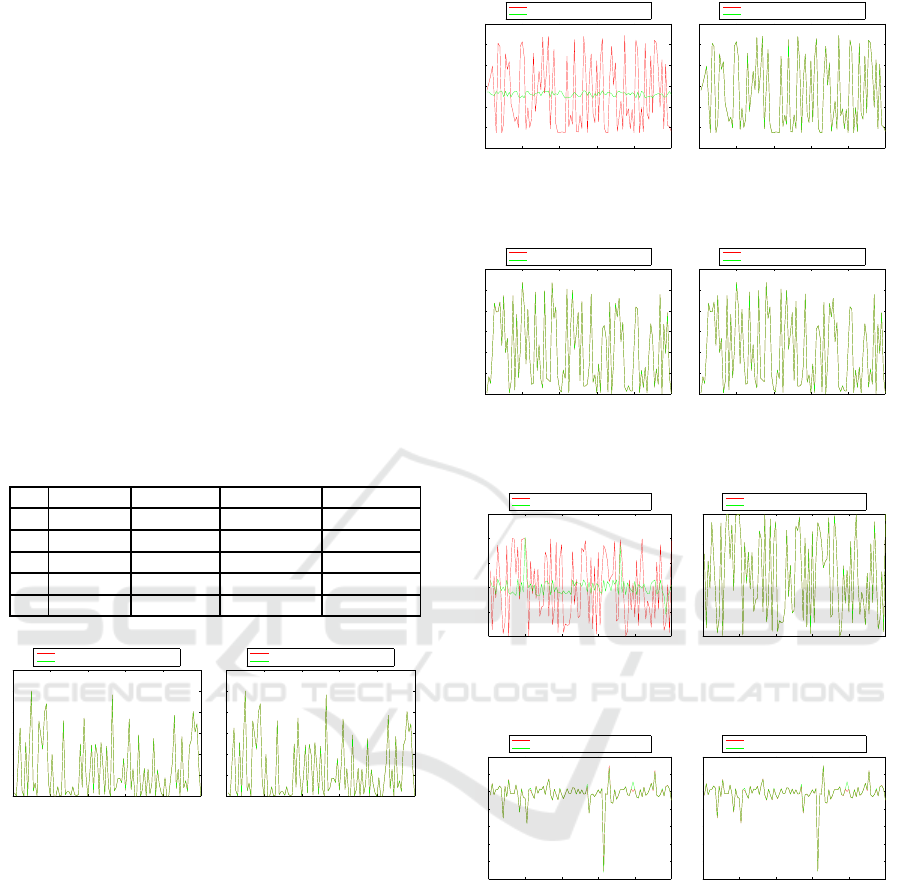
5.1.2 Results in Benchmark Data
In this section, we discuss the results obtained for
each benchmark function. Table 2 shows the fitness
value (MSE) of the best solution found for each ge-
netic algorithm, individuals representation and bench-
mark function. According to the results, we can see
that the best genetic algorithm scheme for tree rep-
resentation is the stationary, since the mean square
error is lower than GGA-T in all functions. On the
other hand, the best scheme for SLP representation
is generational genetic algorithm. Equations 8 to 12
show the best expressions found by tree representa-
tion, and equations 13 to 17 with SLP, for functions
f
1
(x) to f
5
(x), respectively. In addition, Figures 12,
13, 14, 15 and 16 show graphically the results of the
best approximation function found. We can see that
the best option to model the behaviour data is a SLP
representation with generational scheme in all func-
tions but f
3
(x) and f
5
(x). However, as Figure 14 and
16, SLP also found the right function approximation.
Since in both cases the SLP algebraic representation
is larger than the obtained using trees, we think that
this increase in the MSE is due to the Simplex method
to approximate the function parameters. On the other
hand, we can see that in some cases (functions f
2
(x)
and f
4
(x)), the tree representation proposals were not
able to find an accurate representation. As a partial
outcome in the preliminary experimentation carried
out in this section, we conclude that SLPs have good
potential to overcome local optima and to achieve bet-
ter solutions than using tree representation, although
the final error in the fitness measure might be affected
by the parameters ¯w estimation algorithm.
F
1
(x) = (x
1
∗ (x
1
∗ x
1
) ∗ (x
1
+ 1))
+ ((x
1
∗ 1) ∗ (x
1
+ 1)) (8)
F
2
(x) = (x
2
− 1425.58)/
((−1100.38/(−1100.38/−1100.38))
− (x
2
/(−1425.58))) (9)
F
3
(x) = ((x
3
+ 2.15) − (1.395/ 1.395))
∗ ((x
3
∗ (1.395∗ 1.395) ∗ 1.395)) (10)
F
4
(x) = ((6.57/(6.57− x
4
))/
(x
4
+ (6.57 + 6.57))) + (x
4
/570.08) (11)
F
5
(x) = (((2.068/2.068)/2.068) − (2.068/x
5
))
/((x
5
− 4.075)/4.075) (12)
F
1
(x) = (x
1
+ ((x
1
∗ x
1
)+
((((x
1
∗ x
1
) ∗ x
1
) ∗ x
1
) + ((x1∗ x
1
) ∗ x
1
)))) (13)
F
2
(x) = (exp((sin((x
2
∗ (− 5)))))) (14)
F
3
(x) = (((−1.85) ∗ x
3
) + (((x
3
+ x
3
)+
(((x
3
+ x
3
) + ((x
3
+ x
3
) − (((((−1.85) ∗ x
3
)
+ ((−1.85) ∗ x
3
)) + x
3
) ∗ x
3
)))
− (x
3
+ x
3
))) + x
3
)) (15)
F
4
(x) = cos(x
4
+ x
4
) (16)
F
5
(x) = (x
5
− (x
5
− ((2.1697+ 2.1697)
/((((x
5
− ((2.1697+ 2.1697)/(x
5
− (2.1697
+ 2.1697))))/(2.1697+ 2.1697)) + x
5
) + x
5
))))
(17)
We emphasize that our goal is to seek an algebraic
expression equivalent to initial functions described
Preliminary Evaluation of Symbolic Regression Methods for Energy Consumption Modelling
45
above, for this reason we do not use a set of test data
to validate our solution, if we find an algebraic expres-
sion equivalent to our initial functions, we could ver-
ify that the solution found is the right one. While SLP
finds algebraic expressions equivalent to the objective
functions, trees sometimes fail. On the other hand,
we used the Student’s statistical test to check if there
are significant differences between the error distribu-
tions of the algorithms (GGA-T versus GGA-SLP and
SGA-T versus SGA-SLP). After applying the statis-
tical test, we obtained a p-value less than 0.05 in all
cases, so that we reject our initial hypothesis (non sig-
nificant differences) and we can ensure that there are
differences between the algorithm for SLP represen-
tation.
In the next section, we apply the proposals SGA-
T and GGA-SLP over a real dataset of consumption
data, to check the behavior of the methods under real
problems with low noise data.
Table 2: Benchmark functions results.
GGA-T SGA-T GGA-SLP SGA-SLP
F
1
7.32E14 2.87E-17 0 2.324E-15
F
2
0.619 0.659 1.81E-26 1.81E-26
F
3
6.94E7 1.74E-24 0.1348 270.62
F
4
0.4366 0.4414 0 0
F
5
9.99E-4 1.55E-4 0.0146 0.044
0 20 40 60 80 100
0
2
4
6
8
10
12
x 10
7
Real data
Approximated data with tree representation
0 20 40 60 80 100
0
2
4
6
8
10
12
x 10
7
Real data
Approximated data with SLP representation
Figure 12: Results for f
1
(x) using trees (left) and SLPs
(right). Red lines are the real data, and green lines the ap-
proximated data.
5.2 Description of the Energy
Consumption Dataset
In this section we analyze the energy consumption
data of a set of public buildings. Here, our goal
is to know the feasibility of using symbolic regres-
sion to infer the relationship between the energy con-
sumption of similar buildings in the same compound,
in the case it exists, and provide an analytical for-
mula that explains such relationship. In this work,
our test bed data come from a Campus of the Uni-
versity of Granada containing 5 buildings. For con-
fidenciality restrictions, we name those buildings as
x
1
,x
2
,x
3
,x
4
,x
5
. We use the available data for all
buildings, measured from 2012 to September of 2015.
0 20 40 60 80 100
0
0.5
1
1.5
2
2.5
3
Real data
Approximated data with tree representation
0 20 40 60 80 100
0
0.5
1
1.5
2
2.5
3
Real data
Approximated data with SLP representation
Figure 13: Results for f
2
(x) using trees (left) and SLPs
(right). Red lines are the real data, and green lines the ap-
proximated data.
0 20 40 60 80 100
0
0.5
1
1.5
2
2.5
3
x 10
4
Real data
Approximated data with tree representation
0 20 40 60 80 100
0
0.5
1
1.5
2
2.5
3
x 10
4
Real data
Approximated data with SLP representation
Figure 14: Results for f
3
(x) using trees (left) and SLPs
(right). Red lines are the real data, and green lines the ap-
proximated data.
0 20 40 60 80 100
−1
−0.5
0
0.5
1
1.5
Real data
Approximated data with tree representation
0 20 40 60 80 100
−1
−0.5
0
0.5
1
Real data
Approximated data with SLP representation
Figure 15: Results for f
4
(x) using trees (left) and SLPs
(right). Red lines are the real data, and green lines the ap-
proximated data.
0 20 40 60 80 100
−1
−0.8
−0.6
−0.4
−0.2
0
0.2
0.4
Real data
Approximated data with tree representation
0 20 40 60 80 100
−1
−0.8
−0.6
−0.4
−0.2
0
0.2
0.4
Real data
Approximated data with SLP representation
Figure 16: Results for f
5
(x) using trees (left) and SLPs
(right). Red lines are the real data, and green lines the ap-
proximated data.
Each building has an energy consumption sensor that
measures energy consumption hourly. In addition,
there is an aggregation node (general counter) that
provides the sum of the energy consumption of the
buildings x
1
,x
2
,x
3
,x
4
. Thus, our initial hipothesis
to test is that the value of the general counter y =
x
1
+ x
2
+ x
3
+ x
4
+ ε, where ε stands for an error com-
ing from data preprocessing. We will use symbolic
regression with algorithms SGA-T and GGA-SLP to
test if the methods are able to find such relationship,
to validate the feasibility of the technique to be used
in energy consumption data modeling.
ICPRAM 2017 - 6th International Conference on Pattern Recognition Applications and Methods
46
A prior stage of data preprocessing was required
before applying the algorithms. This preprocessing is
the imputation of missing values (Royston, 2004) for
each energy sensor and data alignment (Rhudy, 2014)
. Finally, as the data are provided hourly, we applied
a data aggregation procedure (Patil and Patil, 2010) to
model daily consumption data. Section 5.3 shows the
results after applying symbolic regression in this real
dataset.
For this experimentation with real data consump-
tion we used the following configuration: 200 indi-
viduals for the initial population and 50000 evalua-
tions. Also, we have used the crossover (probability
of 99%) and mutation (probability of 1%) previously
described. Finally, equation 7 is used as function fit-
ness.
5.3 Results in Real Energy
Consumption Data
Using the experimental settings described in the pre-
vious section, we run 30 experiments so that statistical
analyses could be carried out in the results. Table 3
shows the best fitness values (MSE) obtained for each
representation. Again, a generational scheme in our
genetic algorithm with SLP representation has found
a better solution than the tree representation. Also,
the computational time is less in SLP, and the average
fitness along all 30 runnings is lower. Therefore, here
we also prove the power of SLP representation over
the tree representation in real data.
Table 3: Symbolic regression in a real consumption dataset.
Trees SLP
Average Fitness 5.1142e+15 68.9
Better Fitness 102284.034 43.3801
Worse Fitness 372363.908 94.42
Average time (s) 11714.5 8321
Best solution time (s) 60.5 61
The best solution found by SLP is shown in equa-
tion 18. This formula indicates that the general
counter is the sum of the following 4 building plus
a constant. The term cos(X
3
) is irrelevant because its
range is [-1,1] and we may consider this value as a
constant for lower/upper bounds. This constant could
be model a part of an error derived from data prepro-
cessing.
Y = (X
1
+(((24.476+X
4
)+(X
2
+X
3
))+(cos(X
3
))))
(18)
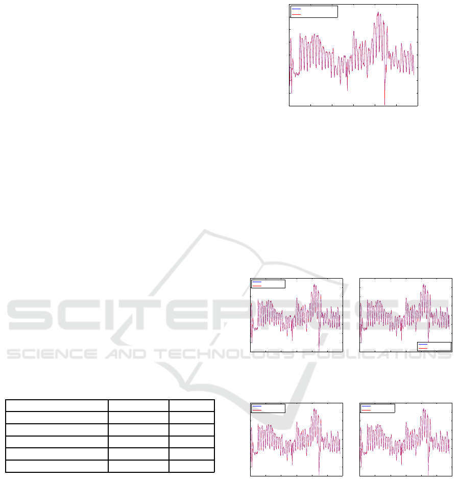
Finally, figure 17 shows in blue the real consump-
tion data, and in red the estimated values with the
0 50 100 150 200 250 300
5500
6000
6500
7000
7500
8000
8500
9000
9500
General counter
Estimated values
Figure 17: Real and estimated consumption data.
found expression 18. So we accept the initial hypoth-
esis to test the inference capabilities of symbolic re-
gression for energy consumption data. The general
counter has been correctly modeled using the infor-
mation from buildings x
1
,x
2
,x
3
,x
4
, and the algorithm
has been able to distinguish that x
5
is irrelevant for
the problem. This fact opens a future research to test
if symbolic regression could be used for both energy
consumption modelling and feature selection, if it is
applied over a larger dataset and more complex initial
hypotheses.
0 50 100 150 200 250 300
5500
6000
6500
7000
7500
8000
8500
9000
9500
Real values
Estimated values
0 50 100 150 200 250 300
5500
6000
6500
7000
7500
8000
8500
9000
9500
Real values
Estimated values
Figure 18: Scatterplots of real data (blue) and estimated
data (red) for the buildings X
1
and X
2
against the general
counter).
0 50 100 150 200 250 300
5500
6000
6500
7000
7500
8000
8500
9000
9500
Real values
Estimated values
0 50 100 150 200 250 300
5500
6000
6500
7000
7500
8000
8500
9000
9500
Real values
Estimated values
Figure 19: Scatterplots of real data (blue) and estimated
data (red) for the buildings X
3
and X
4
against the general
counter.
In order to validate the rightfulness of the result-
ing formula, in case we would have not known the
initial hypothesis in advance, Figures 18, 19 and 20
shows the scatterplots of the general counter against
the other buildings: These figures contain the real and
the estimate data with the resulting formula in 18. In
blue color, we can see the values of real consumption
of the general counter against other building, and in
red color we can see the estimated values by the for-
mula. From these results we can conclude that the
Preliminary Evaluation of Symbolic Regression Methods for Energy Consumption Modelling
47

0 50 100 150 200 250 300
5500
6000
6500
7000
7500
8000
8500
9000
9500
Real values
Estimated values
Figure 20: Scatterplots of real data (blue) and estimated
data (red) for the building X
5
against the general counter.
last building (20) is not providing consumption data
in the general counter, because we have modeled their
consumption with an algebraic e xpression that does
not consider this building, and also that the scatterplot
of estimated data is very accurate being compared to
the initial real data. Thus, as this behavior is fulfilled
in all buildings, we conclude that the resulting for-
mula obtained by symbolic regression is appropriate
to model the consumption data.
6 CONCLUSIONS
In this paper, we have tested the feasibility of using a
new representation in genetic programming: straight
line programs. This alternative to solve the symbolic
regression problem allows an improvement in compu-
tational time due to their linear structure which facil-
itates reuse of algebraic subexpressions, so the search
space is lower in our genetic algorithm and can over-
come local optima. On the other hand, we highlight
the good performance in multivariate problems, being
able to select the relevant variable of the problem in
the real data in our experimentation.
As a general conclusion, we summarize that our
findings suggest that SLP representation has a good
potential as symbolic regression representation mech-
anism, against the traditional tree representation. In
the benchmark data, we have found out that the
method to estimate the parameters during the fitness
evaluation stage could be improved, since it affects di-
rectly to the fitness performance and might hide good
alternative algebraic expressions. In a future work,
we will address this problem by testing other mecha-
nisms for parameter estimation, and also reducing the
size of the resulting SLP expression. Regarding en-
ergy consumption, we will increase our test bed data
and make experimentations with large datasets con-
taining several buildings where an initial algebraic ex-
pression hypothesis cannot be provided in advance to
test the results.
ACKNOWLEDGEMENTS
This work has been supported by the research project
TIN201564776-C3-1-R, Government of Spain. We
thank reviewers for their constructive comments and
useful ideas for future works.
REFERENCES
Alcazar, A. I. E. and Sharman, K. C. (1996). Some appli-
cations of genetic programming in digital signal pro-
cessing.
Alonso, C. L., Monta˜na, J. L., Puente, J., and Borges, C. E.
(2009). A new linear genetic programming approach
based on straight line programs: Some theoretical and
experimental aspects. International Journal on Artifi-
cial Intelligence Tools, 18(5):757–781.
Benz, F. and K¨otzing, T. (2013). An effective heuristic for
the smallest grammar problem. In Proc. of GECCO
(Genetic and evolutionary computation), pages 487–
494.
Berkowitz, S. J. (1984). On computing the determinant in
small parallel time using a small number of proces-
sors. Inf. Process. Lett., 18(3):147–150.
Davidson, J. W., Savic, D. A., and Walters, G. A. (2001).
Symbolic and numerical regression: experiments and
applications. In John, R. and Birkenhead, R., editors,
Developments in Soft Computing, pages 175–182, De
Montfort University, Leicester, UK. Physica Verlag.
Duffy, J. and Engle-Warnick, J. (2002). Using Symbolic Re-
gression to Infer Strategies from Experimental Data,
pages 61–82. Physica-Verlag HD, Heidelberg.
Giusti, M., Heintz, J., Morais, J., Morgenstem, J., and
Pardo, L. (1998). Straight-line programs in geomet-
ric elimination theory. Journal of Pure and Applied
Algebra, 124(1):101 – 146.
K., M. and K., K. (1989). Nonlinear least-squares regres-
sion analysis by a simplex method using differential
equations containing michaelis-menten type rate con-
stants. pages 25–34.
Koza, J. R. (1994). Genetic programming ii: Automatic
discovery of reusable subprograms. Cambridge, MA,
USA.
Krick, T. (2002). Straight-line programs in polynomial
equation solving.
Langdon, W. B. (1998). Genetic Programming — Comput-
ers Using “Natural Selection” to Generate Programs,
pages 9–42. Springer US, Boston, MA.
Lankhorst, M. M. (1994). Breeding grammars: Grammati-
cal inference with a genetic algorithm. In Proceedings
of the 1994 Eurosim Conference on Massively Paral-
lel Processing Applications and Development, pages
423–430. Elsevier.
Lazarus, C. and Hu, H. (2001). Using genetic programming
to evolve robot behaviours.
M., R. A. (2007). Programacin gentica: La regresin sim-
blica. Entramado, 3:76–85.
ICPRAM 2017 - 6th International Conference on Pattern Recognition Applications and Methods
48

Maros, S., Arias Caete, M., and Dominique, R. (2016). En-
ergy efficiency .saving energy, saving money.
McKay, B., Willis, M., and Barton, G. (1997). Steady-state
modelling of chemical process systems using genetic
programming. Computers & Chemical Engineering,
21(9):981 – 996.
McKay, B., Willis, M. J., and Barton, G. W. (1995). Using a
tree structured genetic algorithm to perform symbolic
regression. pages 487–492.
Molina-Solana, M. (2014). Data mining for building energy
management. In Proceedings of Sustainable Places
2014.
Molina-Solana, M., Ros, M., Martn-Bautista, M. J., and
Vila, A. (2014). Minera de datos y gestin energtica:
tendencias actuales. In Proc. XVII Congreso Espaol
sobre Tecnologas y Lgica Fuzzy (ESTYLF2014), pages
627–632.
Naoki, M., McKay, B., Xuan, N., Daryl, E., and Takeuchi,
S. (2009). A New Method for Simplifying Algebraic
Expressions in Genetic Programming Called Equiva-
lent Decision Simplification, pages 171–178. Springer
Berlin Heidelberg, Berlin, Heidelberg.
Neves, S. and Araujo, F. (2015). Straight-line programs
for fast sparse matrix-vector multiplication. Concur-
rency and Computation: Practice and Experience,
27(13):3245–3261.
Pan, J., Jain, R., and Paul, S. (2014). A survey of energy ef-
ficiency in buildings and microgrids using networking
technologies. IEEE Communications Surveys Tutori-
als, 16(3):1709–1731.
Pandey, H. M. (2016). Performance evaluation of selec-
tion methods of genetic algorithm and network secu-
rity concerns. Procedia Computer Science, 78:13 –
18.
Patil, N. S. and Patil, P. P. R. (2010). Data aggregation in
wireless sensor network.
Rhudy, M. (2014). Time alignment techniques for experi-
mental sensor data. volume 5.
Royston, P. (2004). Multiple imputation of missing values.
volume 4.
Schmidt, M. and Lipson, H. (2010). Symbolic Regression
of Implicit Equations, pages 73–85. Springer US,
Boston, MA.
Sequera, J., del Castillo Diez, J., and Sotos, L. (2012). Doc-
ument clustering with evolutionary systems through
straight-line programs slp. Intelligent Learning Sys-
tems and Applications, 4(4):303–318.
Tsoulos, I. G. and Lagaris, I. E. (2006). Solving differ-
ential equations with genetic programming. Genetic
Programming and Evolvable Machines, 7(1):33–54.
Yu, Z., Haghighat, F., Fung, B. C., and Yoshino, H. (2010).
A decision tree method for building energy demand
modeling. Energy and Buildings, 42(10):1637 – 1646.
Preliminary Evaluation of Symbolic Regression Methods for Energy Consumption Modelling
49
