
Transportation-based Visualization of Energy Conversion
Oliver Fernandes, Steffen Frey and Thomas Ertl
VISUS, University of Stuttgart, Allmandring 19, Stuttgart, Germany
Keywords:
Energy Transport, Glyph-based Visualization, Glyph Placement, Volume Rendering, Energy Flux, Flow
Dynamics.
Abstract:
We present a novel technique to visualize the transport of and conversion between internal and kinetic energy
in compressible flow data. While the distribution of energy can be directly derived from flow state variables
(e.g., velocity, pressure and temperature) for each time step individually, there is no information regarding
the involved transportation and conversion processes. To visualize these, we model the energy transportation
problem as a graph that can be solved by a minimum cost flow algorithm, inherently respecting energy con-
servation. In doing this, we explicitly consider various simulation parameters like boundary conditions and
energy transport mechanisms. Based on the resulting flux, we then derive a local measure for the conversion
between energy forms using the distribution of internal and kinetic energy. To examine this data, we em-
ploy different visual mapping techniques that are specifically targeted towards different research questions.
In particular, we introduce glyphs for visualizing local energy transport, which we place adaptively based on
conversion rates to mitigate issues due to clutter and occlusion. We finally evaluate our approach by means of
data sets from different simulation codes and feedback by a domain scientist.
1 INTRODUCTION
With the ever growing computational power avail-
able, flow simulations performed by scientists and en-
gineers become more realistic and detailed. There-
fore, the analysis of occurring flow phenomena be-
comes increasingly difficult, and available tools may
not be adequate to the task. New visualization tech-
niques are necessary to be able to explore the dif-
ferent aspects of phenomena occurring in the data.
In particular, the consideration of conserved quanti-
ties proves to be a valuable asset in both mathemat-
ics and physics, and is ultimately fundamental for our
understanding of nature. Used as a basis for model-
ing flow dynamics, the conservation laws of physics
are employed to establish a set of partial differential
equations to describe the dynamics of a fluid in mo-
tion. Basically, this is done by first determining the
composition of a conserved quantity, and identifying
its constituents. The different ways the quantity can
change over time is then examined by modeling ap-
propriate physical interactions. The quantity needs to
be analyzed in a temporal context, as only examining
a given state of the simulation, even when considering
all defining variables, may not reveal all dynamics in-
volved. For example, the visualization of the velocity
does not suffice to fully understand the dynamics (i.e.
transport) of momentum for the simple case of an in-
compressible steady laminar flow simulation. In this
particular case, the solution is fairly simple: by taking
into account the deviatoric stress tensor, the true mo-
mentum flux field can be derived for each component,
and analyzed via standard vector field visualization.
However, this is not the case in general. Usually,
all dynamics calculated by solving the partial differ-
ential equations cannot be extracted directly from the
state of the fluid. In a more interesting example of a
compressible flow simulation, one cannot directly de-
rive, given the initial and final state of the fluid, how
an energy change has occurred. The final state can,
in theory, be reached by various combinations of ex-
changing heat or having work done on its volume.
In this paper, we propose an approach to visualize
this process for arbitrary flow data by examining the
exchange of total energy between control volumes.
The resulting energy flux is in turn used to compare
the composition of energy types in the initial state
with the final state. Based on this comparison, a visual
representation is generated showing the spatial distri-
bution for the conversion between different forms of
energy.
In Sec. 2 we give an overview on related work. Af-
ter providing a quick outline of our overall approach
and describing the underlying fundamentals regard-
52
Fernandes O., Frey S. and Ertl T.
Transportation-based Visualization of Energy Conversion.
DOI: 10.5220/0006098200520063
In Proceedings of the 12th International Joint Conference on Computer Vision, Imaging and Computer Graphics Theory and Applications (VISIGRAPP 2017), pages 52-63
ISBN: 978-989-758-228-8
Copyright
c
2017 by SCITEPRESS – Science and Technology Publications, Lda. All rights reserved

ing energy densities occurring in flow (Sec. 3), we
then discuss and evaluate the individual components
of our approach, which we consider to be the main
contributions of our paper:
• We introduce our approach to estimate energy
conversion for visualization by reformulating and
solving it as a transportation problem (Sec. 4).
• We then discuss several mapping approaches for
the visualized quantity to generate meaningful
renderings from the obtained energy data (Sec. 5).
• We evaluate the utility of our approach with dif-
ferent data sets and an expert study with a domain
scientist (Sec. 6).
We finally conclude our work in Sec. 7.
2 RELATED WORK
Since the visualization of energy and energy transport
can lead to significant insights of the explored data
set, a few approaches to the problem have been sug-
gested. However the intricate nature of the problem,
both theoretically and technically, proves it to be a
difficult task to produce a concise and comprehensive
visualization of all the information contained.
Many visualization techniques to explore flow
data have been developed over the years. Relevant for
the approach discussed in this paper are several prior
works, relating to various steps of our approach.
Already in 1905, visualizing the participation of
energy in an experiment or a simulation, often so-
called Sankey diagrams were (Sankey, 1905) (and still
are) used, to give an abstracted overview of energy ex-
change. Of course, any further information regarding
the spatial distribution is lost.
Many geometry-based techniques have been de-
rived processing the underlying fields of the data
to generate geometry representing its characteristics.
Among these are the well-known streamlines and
similar integration techniques resulting in geome-
try, which resemble the velocity vector field of the
flow. For an overview of geometric visualizations, see
(McLoughlin et al., 2010).
Often a mixture of texture-based and geometry-
based approach already reveals much information
about the flow, for example done with LIC on isosur-
faces in (Laramee et al., 2004). An extension of these
are stream tubes, which are densely seeded stream-
lines on a closed curve, therefore creating a tube-like
structure (Schroeder et al., 1991). Various improve-
ments have been made to enhance the usage of stream
tubes, for example (McLoughlin et al., 2013). An
interesting property of these is that there is no flow
across the tube mantle (per definition). In this con-
text, Meyers and Meneveau (Meyers and Meneveau,
2012) suggested so-called energy transport tubes to
visualize the transport of kinetic energy in statistically
steady flows. Again, defining an energy tube mantle
as the two-dimensional manifold where energy flux
does not have a normal component (i.e. total energy
stays the same summed up across the cross-section
of such a tube), they give a good visualization of the
propagation of kinetic energy. However, they do not
help in exploring phenomena beyond transport of an
energy form. Also, arbitrary sources and sinks can-
not be included as easily. They also do not consider
the different forms of energy present in a flow simula-
tion, and how the composition of the total energy can
reveal additional information about the data.
With our approach aggregating energy transport
information to yield a scalar value for the conversion,
direct visualization techniques need to be considered.
Very common are techniques like volume render-
ing which are used for scalar fields of flow data such
as density. Still being an active part of research, vol-
ume rendering has many applications in scientific vi-
sualization, e.g. (Kroes et al., 2011). Also more
lighting-based techniques can help to present the data
more intuitively, as for example shading cues, em-
ployed in (Boring and Pang, 1996) for vector field
fields, such as the velocity. A good overview of direct
visualization for higher order data, and possible visu-
alization approaches is given in (Sadlo et al., 2011).
Glyphs provide a very good means of visualizing
multivariate and higher order data. Our approach re-
sults in multivariate data represented by a dense graph
of the data set with both nodes and edges having rele-
vant scalar values applied (node count on the order of
cell count). A concise yet intuitive way of interpret-
ing the data is needed. However, for multivariate data,
there is no straightforward standard technique to visu-
alize involved quantities directly. An overview of us-
ing glyphs to represent multivariate data can be found
in (Borgo et al., 2013) and (Ropinski et al., 2011).
Custom glyphs incorporating all dimensions and vari-
ables of the data can be designed, as is done for exam-
ple in vector uncertainty visualizations (Wittenbrink
et al., 1996), where the classic “hedgehog” vector
field visualization is enhanced with additional infor-
mation on the uncertainty. A novel approach of us-
ing the glyph in a multi-scale fashion, where different
zoom levels of the same dense glyph layout revealed
different information about the data set, was pre-
sented in (Hlawatsch et al., 2011). This also encom-
passes customizing glyphs to fit the underlying data,
as shown in (Kraus and Ertl, 2001) or (Tong et al.,
2016). Glyphs also work well for flow data when con-
Transportation-based Visualization of Energy Conversion
53

sidering the tensors (Jacobian, Hessian) of flow quan-
tity derivatives, and are a popular tool for visualiz-
ing higher order quantities (Schultz and Kindlmann,
2010). An example of combining direct and glyph
visualization in an integrated approach is shown in
(
¨
Uffinger et al., 2011).
Our technique determines the flow of energy be-
tween subsequent time steps to visualize the conver-
sion processes. Conceptually, this is related to the
earth mover’s distance (EMD). Basically, it deter-
mines the minimum cost of turning one distribution
into the other. First, it constructs a complete graph,
taking each cell of the data as a node (i.e., every pair
of nodes is connected by an edge). In our approach,
we use a minimum-cost flow solver to compute the
distance (e.g., (Goldberg and Tarjan, 1990)). In more
detail, we employ a widely used technique in this cat-
egory: the cost-scaling push-relabel algorithm (Gold-
berg and Tarjan, 1986). It maintains a preflow and
gradually converts it into a maximum flow by mov-
ing flow locally between neighboring vertices using
push operations under the guidance of an admissible
network maintained by relabel operations. This algo-
rithm will find an optimal solution (i.e., one with min-
imal associated cost). In this paper, we use Google’s
implementation of this algorithm
1
. Its complexity is
O(n
2
· m · log(n · c)), where n denotes the number of
nodes in the graph, m denotes the number of edges,
and c is the value of the largest induced edge cost in
the graph. Due to this comparably high complexity,
we exploit certain properties, particularly to signif-
icantly reduce the number of edges to make its di-
rect application to cells of a data set computation-
ally feasible. The EMD is particularly popular in the
computer vision community where distances are typ-
ically computed between color histograms, e.g., for
image retrieval (Rubner et al., 2000). To interpolate
between commonly used distributions in computer
graphics (like BRDFs, environment maps, stipple pat-
terns, etc.), Bonneel et al. (Bonneel et al., 2011) de-
compose distributions into radial basis functions, and
then apply partial transport that independently consid-
ers different frequency bands.
3 MOTIVATION AND
FUNDAMENTALS
In this section, we give a quick overview of the prob-
lem determining the transport of total energy for visu-
alization within a given domain, and outline our ap-
proach to solve this problem. We then give a short
1
https://developers.google.com/optimization
introduction to the relevant fundamentals of energy in
fluid dynamics. The section concludes with a brief
summary of the minimum cost flow algorithm.
3.1 Motivation for Visualizing Energy
Transport
Any process can be divided into variables describing
the state, e.g. velocity, pressure etc., and variables de-
scribing the dynamics as for example various fluxes.
The energy transport we aim to visualize in this pa-
per, can be classified as pertaining to the dynamics of
any flow. However, these dynamics involved propa-
gating the system between states cannot be easily ex-
tracted in an arbitrary flow, but enable useful insights,
as for example, predictions for the evolution of the
system. In real life phenomena, dynamical data of-
ten cannot be captured, and is unavailable for analysis
(e.g. momentum exchange in global weather air flow
data). Using computational fluid dynamics, the evo-
lution equations (Navier-Stokes equations, see sec-
tion 3.2) modeling the flow are known. Even so, there
are various approaches to discretize and solve these
equations, possibly leading to the resulting dynamics
being difficult to extract from the calculation. Even
if possible, doing this highly depends on the type of
simulation and solver (e.g., implicit or explicit), as
well as the respective implementation. In all cases,
retrieving the state variables is fairly easy.
Our approach estimates the energy dynamics of
any arbitrary system, for which the state variables
are known at different time steps (Sec. 4). One of
the two prerequisites necessary for the employed al-
gorithm is to know how the amount of energy in a
given energy form is related to the state variables of
the system. The other prerequisite is information re-
garding all additional external sources and sinks (or
an approximation thereof), to satisfy the energy con-
servation law. The composition of the total energy,
i.e., the types of energy involved, may be chosen arbi-
trarily for our calculation. This is an important prop-
erty of our approach in that it is widely applicable to
data from many kinds of sources. In particular, using
only an initial and final state, knowledge of the ac-
tual evolution equations, which, as explained above,
might not always be available, are not necessary to
compute the energy dynamics. However, any addi-
tional knowledge of the domain, or knowledge of the
transport mechanisms, can be included to improve the
accuracy of the estimated energy fluxes.
To render the myriad of energy flux information
yielded by our visualization, we discuss several map-
pings for the data in Sec. 5). These include a vol-
ume rendering for exploration and overview, as well
IVAPP 2017 - International Conference on Information Visualization Theory and Applications
54

as a glyph-based approach. The glyph approach is
further enhanced by automatically placing the glyphs
for minimal occlusion, while retaining the most im-
portant information.
3.2 Energy in Fluid Dynamics
Several forms of energy are present in a compress-
ible flow data set. First, there is kinetic energy, for
any mass moving at a non-zero velocity. Other kinds
of energy include internal energy, a thermodynami-
cal quantity dependent on the pressure and tempera-
ture. While we focus on these two types of energy,
various other forms of energy can effortlessly be con-
sidered and implemented in a straight forward fash-
ion. In the following, we give a brief overview of the
partial differential equations governing compressible
flow. We also give a quick summary of the energy
types involved and their calculation.
Being independent of underlying governing equa-
tions, we only need to consider the forms of energy
present in a given data set, regardless how the data
was actually produced. For the data sets in this pa-
per, this specifically means considering the internal
and kinetic energy forms. For all known phenom-
ena in compressible flow, the Navier-Stokes equations
(NSE, 1) prove a very accurate and general model
(Hasert, 2014; Landau and Lifshitz, 1987).
Derived from basic conservation equations for
mass, momentum and energy (yielding (1a), (1b) and
(1c) respectively), the compressible NSE take the fol-
lowing form:
∂
t
ρ + ∇· (ρu) = 0 (1a)
∂
t
(ρu) + ∇ · (ρu ⊗ u + pI) = ∇ · σ
0
(1b)
∂
t
(ρε) + ∇ · (ρu(ε + p)) = ∇ · (σ
0
· u) − ∇ · q − B
(1c)
p = ρRT, (1d)
where ρ is the mass density, u the velocity, p the pres-
sure and T the temperature. ε denotes the specific
energy per unit mass (i.e. the energy density), and
σ
0
the deviatoric stress tensor. q is the the heat flux.
The final equation closing the set is the equation of
state for an ideal gas (1d), using the gas constant R.
B is the sum of conservative external fields. However,
for numerically solving this set of partial differential
equation, various terms need to be approximated and
modeled accordingly. In some cases, the exact mod-
eling may not be available, as for measured data. The
energy conservation is expressed in terms of the spe-
cific energy per mass unit ε:
ε = e +
1
2
|u|
2
. (2)
e = c
v
T is the internal energy. Multiplication with ρ
defines an energy density e
tot
. In the following, the
term energy will be used synonymous to energy den-
sity for brevity.
Using the NSE as a basis, the types of energy occur-
ring in compressible flow can be derived. A given
energy distribution can be split into several distinct
parts. For one, there is the internal energy given by
e
int
= ρc
v
T with the heat capacity c
v
at constant vol-
ume. The heat capacity c
v
can be expressed with a
material parameter, the adiabatic index constant γ, as
c
v
= R/(γ−1), finally yielding an internal and kinetic
energy of
e
int
=
ρT
γ − 1
(3)
e
kin
=
1
2
ρ|u|
2
(4)
Other forms could also be taken into considera-
tion, for example potential energy in external fields B,
given with e
pot
= ρgz.
The NSE as expressed in (1), do not encompass
all possible flow physical phenomena. Various exten-
sion (e.g. Magnetohydrodynamics, which also con-
sider the Maxwell equations (Goedbloed and Poedts,
2004)) can be found, possibly adding further forms
of energy to the composition of the total energy. The
data sets considered in this paper focus on the inter-
nal and kinetic energy, and assume no external fields.
In any case, the conserved quantity is the total en-
ergy e
tot
, given by the sum of all the occurring energy
types. For the cases considered in this paper, this is
simply given by e
tot
= e
kin
+ e
int
.
To fully describe the flow problem, or more
specifically the energy conservation problem, the sys-
tem needs to be closed, or the interaction with the
surrounding environment must be considered. This
is usually done by restricting measurements or sim-
ulation to a certain domain, for which the boundary
conditions are known or can be modeled sufficiently.
3.3 Minimum Cost Flow Problem
On the basis that energy only gets exchanged in a
close neighborhood of a cell, we formulate our en-
ergy exchange with a minimum cost flow problem. In
this subsection, we give a brief summary of this algo-
rithm and its terminology.
A minimum cost flow problem examines the trans-
port of a scalar quantity through a network, defined by
a graph G. Two sets of nodes are given: a source set
S and a destination set D. All nodes s,d in S,D are
assigned an integral scalar value s
Q
,d
Q
called supply
and demand respectively. The supply and demand for
each node in S,D must be chosen so that
∑
S
s
Q
= −
∑
D
d
Q
. (5)
Transportation-based Visualization of Energy Conversion
55

Equation 5 expresses that the quantity in question is
preserved. A graph connecting the two sets is estab-
lished by creating a set E of directed edges between
source nodes and destination nodes. Only connec-
tions from S to D are allowed, connections back or
within S or D are disallowed. S,D and E make up the
graph G which defines the input for a minimum cost
flow algorithm.
The problem now consists of moving supply from
S to D, that is, assigning a set of so-called ’flow’ val-
ues f
e
for each edge e, so that:
∀s ∈ S : −
∑
f ∈I
f = s
Q
, I = { f
e
| e starts at s}
∀d ∈ D :
∑
f ∈I
f = d
Q
, I = { f
e
| e ends in d}
(6)
In simple terms, this means that all the supply needs to
be transported to cover all the demand, and can only
be moved along an edge defined in E. No source node
can distribute more than it has supply, and no destina-
tion node can receive more than it has demand.
This condition alone potentially still allows a myr-
iad of solutions. To further limit the possibilities, a
more specific one can be selected by introducing a
secondary condition. This requires assigning a cost c
e
to every edge e in E, which can be arbitrarily adjusted.
With the assignment of c
e
, the selected solution must
additionally minimize the so-called total cost c
T
:
c
T
=
∑
e∈E
f
e
c
e
(7)
The cost value c
e
can be lowered for certain edges to
favor these edges being chosen to move the supply
quantity.
4 EXTRACTION OF ENERGY
TRANSPORT
To enable a comprehensive visualization of the en-
ergy dynamics, we first need to extract the appropriate
quantities. The second part is to map these quantities
to a renderable representation, explained in Sec. 5.
Initially, the value for the two relevant energy den-
sities from the state variables, employing equations
3 and 4, is calculated. After determining the energy
contained in each cell for two consecutive time steps,
we calculate an approximation of the flux for the to-
tal energy e
tot
between the two time steps. Since the
quantity is conserved, the total change of the energy
in the domain between time steps can be determined
by taking the initial total energy and considering all
additions and subtractions at the domain boundary
(Reynolds transport theorem (Leal, 2007)).
Obviously energy changes can only be transported
by a mechanism (i.e. energy itself does not have
a ’speed’), and therefore the limiting speed of this
mechanism also limits the distance energy can be
moved. For a sufficiently small time step, this trans-
port can be assumed to only occur within a small
neighborhood for each cell. This extraction step
“splits off” the energy transport information and pre-
pares it to be mapped to an appropriate visual repre-
sentation. In the following paragraphs, we reformu-
late our problem of determining the energy flow as
a transportation problem. The outcome can then be
directly processed by a standard minimum cost flow
solver to eventually calculate the energy flux.
For the rest of this discussion, the term energy
refers to the total energy density. Matching the en-
ergy flux problem to be solvable by a minimum cost
flow algorithm involves the following steps:
1. Define all cells of the input grid in the first time
step as nodes in S and associate the correct energy
representing the supply s
Q
. Analogously, define
the cells in the second time step as nodes in D
with demand d
Q
.
2. Model the correct boundary conditions for the
nodes in both S and D.
3. Convert the floating point values to integers (re-
quired by the solver), and normalize the energy
to fulfill equation (5) in a distribution-preserving
fashion.
4. Determine an edge set E connecting the two time
steps and solve the defined minimum cost flow
problem. In our setup, we employ the google or-
tools solver to evaluate the minimum cost flow
problem.
In the following paragraphs, we explain these steps in
more detail.
1. Preparing the Energy Data. As an example for
given input data without compromising generality, we
consider the fluid state to be defined by velocity u,
pressure p and temperature T in the following subsec-
tions. The step 1 can be implemented in a straightfor-
ward manner. With the velocity u, the pressure p and
the temperature T provided for each cell by the sim-
ulation, the mass density ρ can be calculated using
equation (1d). Using the mass density, the energies
can be determined with equations (3) and (4), leading
to an energy e
tot
(see section 3.2). With the equation
of state, similar calculations can be done for any set
of state variables.
2. Handling the Boundary Conditions. Modeling
the correct boundary conditions for step 2 is more
complex. In particular, the source and destination
time steps cannot be treated symmetrically: Any
IVAPP 2017 - International Conference on Information Visualization Theory and Applications
56

amount of quantity entering the domain has to be
considered in the source step, while quantity leaving
the domain only applies to the destination time step.
In order to keep the energy conservation assumption
valid, the exchange of energy over the boundaries
must be fully accounted for. This will also ensure
condition (5) is automatically fulfilled.
To correctly map the boundary effects, we need to
identify domain boundaries where energy exchange
is possible. For brevity, we only discuss a few impor-
tant exemplary boundary conditions occurring in our
data sets. A correct modeling for missing (or even
completely different) conditions can be easily derived
based on these ideas.
For each of the state variables u, p and T a bound-
ary condition can be defined as explained in sec-
tion 3.2. Periodic boundaries need to be constructed
with the effect that an addition of energy is modeled
in the source time step S, while the exact same re-
moval is implemented in the destination D for the pe-
riodic neighbor. Dirichlet boundary conditions allow
for both adding and removing energy from the do-
main, depending on the prescribed value and the ac-
tual value of the quantity in the adjacent control vol-
ume. For example an inflow boundary condition (u,
p and T prescribed) can be modeled by adding a cell
(called boundary node) to the source set S for all grid
cells at a location fulfilling the condition (i.e. touch-
ing the inflow boundary), and supplying the state vari-
able according to the prescribed values.
Neumann boundary conditions also may change
the energy contained in the domain. As a prominent
example, consider the outflow boundary condition,
e.g. where derivatives of u, and T are zero, while
the value of p is fixed. The mass flux itself can trans-
port energy out of the domain, and the difference in p
may exchange energy too. The removed energy can
be calculated taking the amount of mass crossing the
boundary (scalar product of mass flux and boundary
normal), while the pressure is set to the fixed value of
the simulation parameter. Now the associated energy
can be calculated and, just as for the inflow condition,
a set of additional cells (i.e. boundary nodes) need to
be added into the destination set D, to be used with the
calculated energy. For different combinations of Peri-
odic, Dirichlet and Neumann conditions for the state
variables, the calculation of energy exchange must be
accounted for individually. Some boundary condi-
tions do not allow for an exchange in the first place,
and therefore do not require a special treatment.
Fig. 1(b) shows a schematic of a cross section of
our beam in cross flow data set. The gray boxes indi-
cate areas, to which energy exchange is possible, and
needs to be handled by boundary nodes. Note that
only the connectivity to the data set and energy den-
sity of these boundary nodes is needed, the geometry
is irrelevant.
3. Normalization and Quantization. After prop-
erly setting up the energy distributions in the previ-
ous steps, the rescaling and quantizing step 3 is per-
formed, to fulfill equation 5 and to turn the floating
point energy to an integral supply/demand value for
the minimum cost flow algorithm. This involves sim-
ply multiplying all energy values by a fixed value and
rounding down the result to the closest integer.
This quantization, and numerical precision issues, or
even insufficiently accurate modeling or estimation of
the boundary condition, can cause the precondition
(5) to fail. To remedy the problem, a normalization
is done to adjust the higher total domain energy to
the lower one. Simply scaling all values by a con-
stant factor (the ratio of the total domain energies) is
not possible, since the energy values are already quan-
tized. Instead, a unit of supply/demand from a node
in the set with the higher total domain energy is re-
moved in a random fashion, until both time steps con-
tain the same accumulated total energy. To keep the
overall distribution approximately the same, cells get
selected for removal proportional to their energy con-
tent.
4. Building and Solving the Graph. Now that the
nodes S,D, and associated supply and demand s
Q
,d
Q
,
of the graph have been established, the edge set E can
be constructed in step 4. Following the assumption
at the beginning of this section, that energy can only
propagate to cells within a certain neighborhood, the
edges can be constructed accordingly. For each node
in the source S, a neighborhood set is selected in the
destination set D based on spatial proximity. Fig. 1(a)
shows the most simple subgraph for a single desti-
nation cell (blue). This cell can potentially receive
an energy flow from the source cells (framed in red)
located in the neighborhood. The figure only shows
immediate neighbors in two dimensions for simplic-
ity, and may actually be an arbitrary unstructured grid
in three dimensions with connection to further neigh-
bors in addition to the nearest. The neighborhood
to which edges are constructed, is determined by a
face-neighbor relationship, and recursive collection of
nearby cells, until a certain maximum distance from
the original cell is achieved.
This distance is determined by the maximum
speed at which a mechanism can transport energy,
multiplied by a constant factor, to account for errors
introduced in the quantization/normalization step.
This can happen when the algorithm is forced to move
a unit of energy further than it could have propagated
physically, and can be controlled by the edge cost c
e
Transportation-based Visualization of Energy Conversion
57
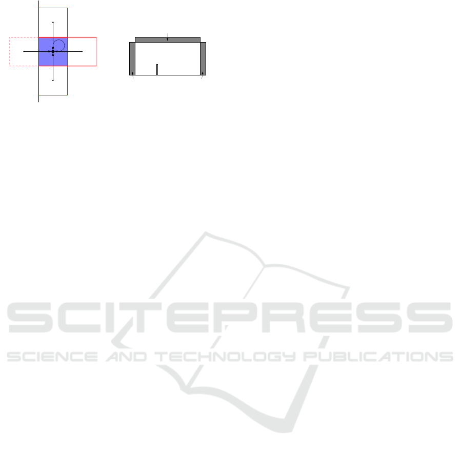
Boundary
(a) Simplified minimum
cost flow subgraph for a
single cell (blue) and con-
nected source cells (red).
Inflow Outflow
Outflow
(b) Boundary conditions
example, here for the
beam in cross flow data
set.
Figure 1: Establishing the minimum cost flow network
graph, and how boundaries are considered.
(see below). Note that a cell’s source node has an
edge to the same cell’s destination node. A boundary
node, depicted in Fig. 1(a) with a dashed red line, is
only connected to it’s adjacent “spawning” node.
All edges e in the set E get assigned a cost c
e
based
on Euclidian distance between the cell centers. There-
fore, the actual geometry of boundary nodes is arbi-
trary, since the boundary node only has a single edge,
connecting it to the source/destination cell in the data
domain to which it injects, or from which it removes
energy, respectively, and must fulfill equation (6). We
promote the use of shorter edges, based on the fact
that the physical energy transport is continuous, and
the assumption that the time interval between time
steps is very small. We do this by defining the edge
cost c
e
using the squared Euclidian norm on the vec-
tor connecting the cell centers s,d: c
e
= ks − dk
2
.
With construction of the edge set E the energy
transport has been fully mapped to a minimum cost
flow problem. To solve the problem, we employ a
generic minimum cost flow algorithm with the prop-
erty of finding an optimal solution, in the sense that
the total cost c
T
(see equation (7)) for this solution is
a global minimum for all possible solutions.
By executing the minimum cost flow algorithm on
the graph G a flow value f
e
for each edge in E is de-
termined. These flow values can be interpreted as the
energy needed to be transported from starting (source)
nodes to ending (destination) nodes, to achieve the en-
ergy distribution in the second time step starting from
the first. In addition, the total cost c
T
for the gener-
ated solution can be interpreted as a coarse indicator
for the accuracy of the approximation.
5 VISUAL MAPPING OF ENERGY
TRANSPORT QUANTITIES
Obviously, the representation provided by the min-
imum cost flow algorithm cannot be displayed in a
straightforward manner, since the graph G is usually
very dense. Even when considering the fact that the
outflow values from source nodes contain the same in-
formation as the inflow values from destination nodes
(only sorted differently) there is still too much infor-
mation per cell. For each destination cell for example,
there can be several (incident) edges, of which each
in turn carries two relevant scalar values, the energy
distribution s
r
(e.g. encoded in the ratio e
int
/e
tot
) in
the source cell, and the energy flow amount f
e
. Addi-
tionally, the destination cells energy ratio d
r
has to be
considered to extract actual conversion information.
We show several approaches which help to explore
the energy conversion under different aspects. These
mappings may also be combined to complement each
other.
5.1 Energy Conversion
First, we define a scalar field giving an overview of
the energy conversion. This field incorporates the
transported amount, as well as the ratios and their spa-
tial distribution over the entire domain. The propaga-
tion direction of energy is lost, however. To calculate
an expressive scalar value C for the conversion, given
the input as explained in the introduction part of this
section, we use a point-based intermediate data repre-
sentation mapping each point to a single scalar.
For our intermediate representation, we construct
a point p
e
for each of the incident edges in the graph
G. The geometry of p
e
is simply the cell center of
the destination node. To define a scalar value C
max
for
each point, we calculate s
r
and d
r
for the source and
destination cells. We then take the absolute value of
the difference between s
r
and d
r
and weight it with
the amount of energy f
e
transported over the edge:
C
max
= ks
r
− d
r
k · f
e
(8)
This yields a scalar for the conversion ratio be-
tween consecutive times in each cell, regardless of
cell geometry or absolute values, while still encoding
all important information.
5.2 Volume Rendering
With Volume Rendering being a good tool to show
spatial distributions, we use it to generate overview
approaches of the energy transport.
IVAPP 2017 - International Conference on Information Visualization Theory and Applications
58
Total Energy Flow Amount. The simplest visualiza-
tion of the energy transport data is summing up the in-
flow of energy f
e
over all incident edges of the graph
for each cell. Displaying this scalar in a volume ren-
dering can give a quick overview of where energy was
transported between cells, and the amount. However,
any directional information, as well as energy compo-
sition information is lost (e.g. Fig. 3(a)).
Direct Conversion Rendering With the Conversion
quantity defined above (Sec. 5.1) being a scalar, a di-
rect volume render can be performed.
Both representations can then be rendered as a com-
mon scalar field as a volume rending. The resulting
scalar field is then rendered by common volume ren-
dering techniques (e.g. Fig. 3(d)).
5.3 Glyph-based Mappings
To preserve the information of local energy transport
on the scale of a cell, we employ glyphs for the mul-
tivariate data.
Transport Glyph. This visualization has the advan-
tage of keeping all the information calculated intact,
including directions of transport, as well as energy ra-
tios. The simplest way of displaying all the graph’s
information is directly showing a subgraph for each
node in a set of selected destination cells.
For every edge from a source cell to the destination
cell, a glyph is constructed. For the energy remain-
ing in the cell, a sphere is drawn, otherwise a cone
is shown, pointing towards the destination cell. The
radius of the sphere, or the cone base respectively, en-
codes the amount of inflow f
e
from the source cell,
while the color shows the conversion ratio. The vi-
sualization enables a detailed examination of energy
flow and conversion for a smaller region. The glyphs
may be placed randomly or manually.
Importance-Weighted Glyph Placement. To avoid
the disadvantages Transport Glyph (occlusion) and
Direct Conversion Rendering (aggregated informa-
tion) have, both variants can be joined into a com-
bined visualization. Based of the conversion ratio
(Sec. 5.1) as an importance weight, cells are selected
as candidates for displaying glyphs. Using a user-
defined threshold for the conversion ratio C
max
, a cell
is added to a set of glyph candidates. Since display-
ing a glyph for all candidates would still lead to mas-
sive occlusion, candidates are then randomly picked
to represent a small neighborhood. The size of this
neighborhood can also be interactively chosen by the
user, offering an overview vs. detail trade-off. This
allows for several valid placement distributions. To
select one, we run the placing algorithm several times,
and keep the distribution with the most glyphs, as this
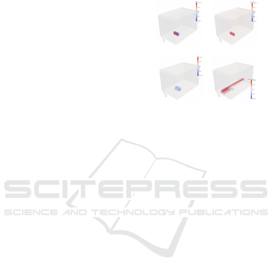
(a) Pressure field (b) Temperature field
(c) Velocity magnitude and streamlines
Figure 2: Volume renderings of the input fields. The images
show the state variables for the beam in cross flow data set
from the destination time step for comparison to our ap-
proach shown in figure 3.
is the one offering the most information. Note that
the glyph distribution can be controlled by any scalar
value as weighting, and may be used in conjunction
with completely different feature detection methods.
6 RESULTS
We employ several flow simulation data sets to dis-
cuss the results achieved with our approach and
demonstrate its utility. These data sets were pro-
duced by different computational fluid solvers. For
the beam in cross flow data set, most simulation pa-
rameters were known, particularly an exact account-
ing for all the boundary conditions of all variables. In
summary, the data consists of an unstructured, time-
varying grid containing 14469 cells. The topology is
constant, and 7 boundary patches are defined. The
state of the fluid is recorded in the velocity, pressure
and temperature. The boundary conditions are set to
appropriate Dirichlet values for the inlet, “slip” for the
side walls, “outflow” for top and back walls, and “no-
slip” for the floor. See below for exact values. For the
5jets data set (provided by K.L. Ma, UC Davis), only
the state variables were available. The data consists
of a regular grid, converted to the corresponding un-
structured mesh consisting of 262144 cells. The state
variables provided are internal energy, density and ve-
locity. We choose the time interval between time steps
to be sufficiently small for our assumptions to apply.
The boundary condition had to be reconstructed by
considering the data close to the boundary, and es-
timating sensible boundary condition types and val-
Transportation-based Visualization of Energy Conversion
59

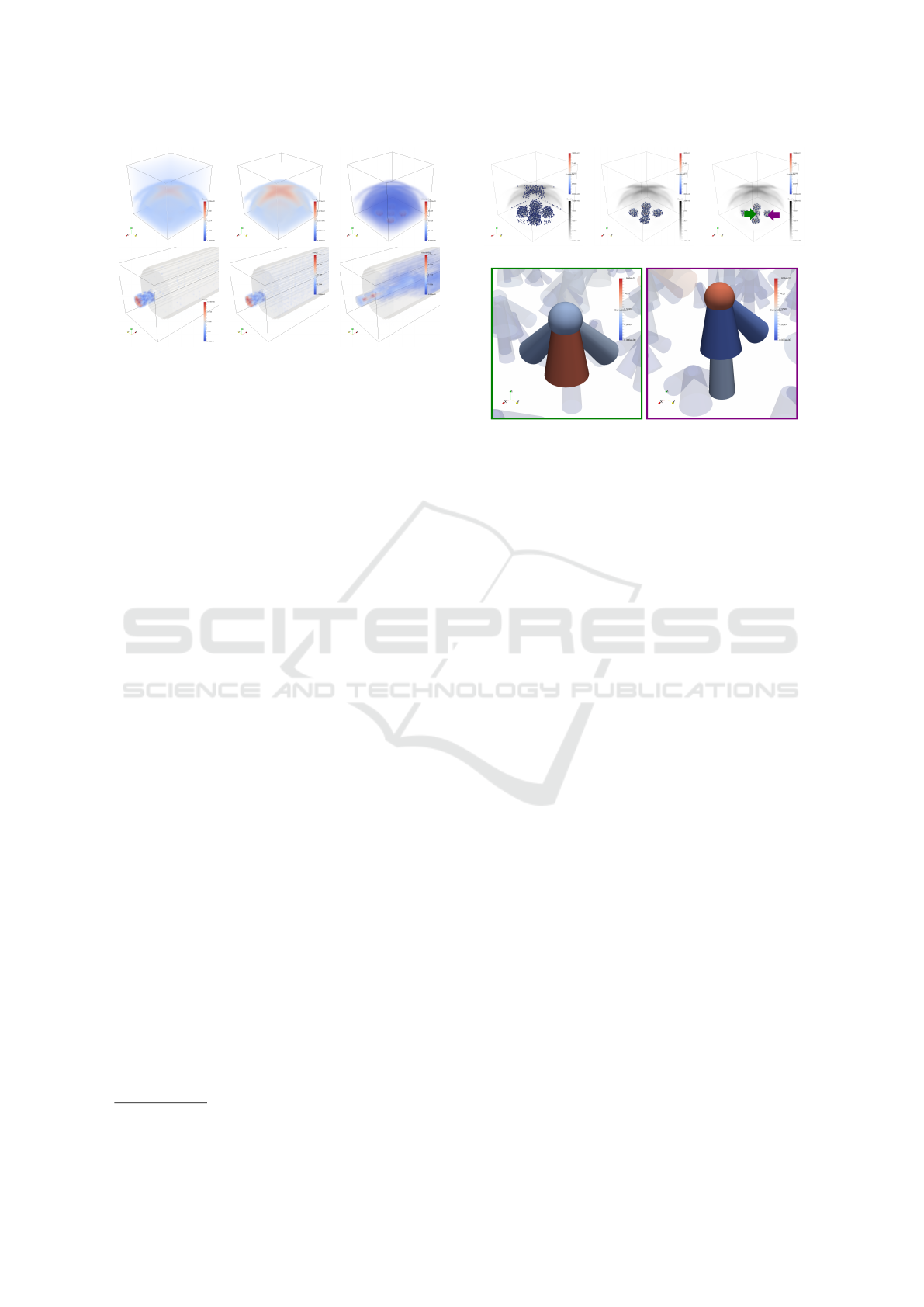
(a) Total Energy Flow (b) Sparse Visualization (c) Zoomed in on structure (d) Conversion
Figure 3: All representations of the energy transport result generated by the minimum cost flow algorithm. (a) The Total
Energy Flow clearly shows the decrease of energy along the x-axis. (b),(c) The Transport Glyph gives a detailed look of
a region of interest (the beam) and the surrounding energy flow including the composition of the energy. (d) Finally, the
Conversion shows the energy exchange between kinetic and internal energy for the entire domain.
ues. For the nozzle data set, all necessary parame-
ters were known and implemented accordingly. De-
tails can be extracted from the publicly available data
set (see Sec. 4). The calculations for the minimum
cost flow algorithm and the subsequent visualization
were performed on an Intel i7-2600K without multi-
threading. In our implementation, we used Google’s
implementation of a minimum cost flow solver to de-
termine the energy flux from our constructed graph.
In the following, we give a short summary of the
data sets, and present our examination results for our
visualization and the implemented mappings in sec-
tions 6.1, 6.2 and 6.3 respectively. We then discuss its
computational performance (section 6.5), and finally
present our expert study (section 6.4).
6.1 Beam in Cross Flow
For this dataset, many of the defining parameters for
the energy transport problem are known, and can be
directly implemented. The foam-extend-3.1
2
pack-
age for flow simulations was used to generate this
simulation data set. It is a fork of the well-known
OpenFOAM package
3
. The constants employed are
p
0
= 100,T
0
= 100,R = 1, γ = 1.4. The images in
Fig. 2 show volume renderings of the pressure, den-
sity and velocity magnitude fields, respectively. We
produced a result for all the representations explained
in Sec. 5, which can be seen in Fig. 3.The image in
Fig. 2(a) shows the Total Energy Flow Amount moved
into a destination cell. One can clearly see the di-
minishing energy transport from the inlet (on the left)
towards the outlet (on the right). This immediately
implies that energy, being only injected on the inlet
boundary condition, dissipates from the domain, at
approximately constant rate. This suggests that the
energy leaves the domain through the top boundary
2
http://www.extend-project.de/
3
http://openfoam.org/
(being an outflow), and the lower boundary (being a
“no-slip” wall). However, this visualization type does
not show a detailed transport of energy, nor any en-
ergy composition information for the region of inter-
est in the data set, the beam structure in the center.
For this, the Transport Glyph can be employed.
The images 3(b) and 3(c) show glyphs depicting
the individual subgraphs for manually selected cells
around the structure. Since in this simple case the
region of interest is known, a manual selection is pos-
sible. The large sphere in the center implies that for
the lower middle part of the structure, not too much
energy is moved, and the small cone pointing into the
sphere shows the small amount of energy entering the
cell. The other cones and spheres can be interpreted
in a similar fashion, and it can be easily seen that the
energy flow is similar to the mass flow. However, con-
sidering Fig. 2(c), differs significantly, as the energy
has other modes of transportation than convection.
The visualization gives a detailed view of the trans-
port for individual cells, and is applicable when the
region of interest is small. Finally, conversion per
cell is rendered in the last figure showing the Energy
Conversion. Employing the volume rendering tech-
nique allows for a complete overview of the whole
domain.
6.2 5jets
For the 5jets data set, the producing parameters are
not known. With our technique, only knowledge of
the boundary conditions is necessary. Information
about the boundary condition can be derived by as-
suming a given boundary condition, and testing if pa-
rameters can be found that match the values on cell
boundaries. After empirically determining the bound-
ary conditions to be outflow on all sides and the top,
and a slip condition for the bottom, as well as 5 cir-
cular patches being the inlets for the jets, we modeled
our setup accordingly. Since the inlet velocity was
IVAPP 2017 - International Conference on Information Visualization Theory and Applications
60
(d) Density (e) Internal energy (f) Momentum
Figure 4: Volume renderings of the input fields using com-
mon visualization techniques. The images show the state
variables for the 5jets (top row) and the nozzle (lower row)
data set from the destination time step for comparison to our
approach shown in Fig. 5 and Fig. 6.
found to vary over time, we also employed further ad-
justments to the empirically determined inlet velocity.
With our approach still being very stable against these
inaccuracies, these assumptions allow for an analysis.
In Fig. 4 we show how the destination time step’s state
variable fields look like in an internal energy, density
and velocity magnitude volume rendering.
Fig. 5 shows the application of the Importance-
Weighted Glyph Placement. A low-opacity volume
rendering of the density for the destination time step
has been added for context. The utility of the (in-
teractively adjustable) conversion threshold parame-
ter C
max
becomes apparent when used to explore the
conversion distribution as a whole, and find areas with
a fairly high (or low) conversion (top row, Fig. 5(a)-
Fig. 5(c)). Zooming in on a high conversion area iden-
tified this way, energy conversion can be examined
per cell. The glyph on the left of Fig. 5(d) receives
a high amount of energy from the cells in the area
below (→ large diameter on cones), only the fraction
transferred from the cell directly below is heavily con-
verted between energy forms (→ saturated red). The
glyph on the right has little conversion and a low in-
flow of total energy from other cells. On the other
hand, the energy remaining in the cell (→ encoded in
sphere), is subject to a fair amount of conversion.
6.3 Nozzle
The nozzle data set, created with OpenLB
4
, is a good
example of a more turbulent simulation. Parameters
defining the simulation can be extracted from the ex-
amples bundled with the solver. In Fig. 4 we show the
destination time step’s state variable fields, similar to
the 5jets data set. For context, the bounding geometry
4
http://optilb.org/openlb/
(a) C
r
= 0.1 (b) C
r
= 0.5 (c) C
r
= 5.0
(d) Detailed glyphs
Figure 5: Energy Conversion glyphs for the 5jets data set for
several conversion thresholds C
max
. (a) - (c) An overview
of the energy conversion can be created by setting a low
threshold. (d) Zooming in, one can adjust the size and den-
sity of the glyphs to reveal the details of the energy flow.
While the conversion for the left cell is heavily influenced
by the energy flow from below, for the cell on the right it
is rather low, with highest conversion taking place for the
energy remaining in the cell.
of the nozzle and tube are shown. Fig. 6 shows a dis-
tribution acquired using Importance-Weighted Glyph
Placement. The density of the glyph coverage as
well as the glyph size can be adjusted interactively
to deal with potential clutter. Both color and opacity
of the glyphs depict the Conversion value. This gives
a good overview of the conversion, and also allows
for a closer examination of the conversion-heavy re-
gions in the center of the nozzle’s jet. The Conversion
(encoded in color) is particularly large right after the
nozzle exit, as well as at the “tip” of the jet. Smaller
cones and spheres at the nozzle imply a small transfer
of energy, indicating that most of the kinetic energy is
converted further along the jet.
6.4 Informal Study
For our study, we interviewed a flow scientist in-
volved in the development of compressible flow
solvers, working as Ph.D. student at TU Delft. On
a daily basis, he uses various visualization tools to
analyze the results. For this task, he develops flow
solver algorithms within the OpenFOAM framework
customized to scalable fluid-structure and fluid-fluid
boundary interaction. He confirmed that the local-
ity assumption for energy transport made in section
4 is valid. For the visualization type showing vol-
ume renderings of the total energy, we showed him
the total energy flow for the beam in cross flow, as
Transportation-based Visualization of Energy Conversion
61
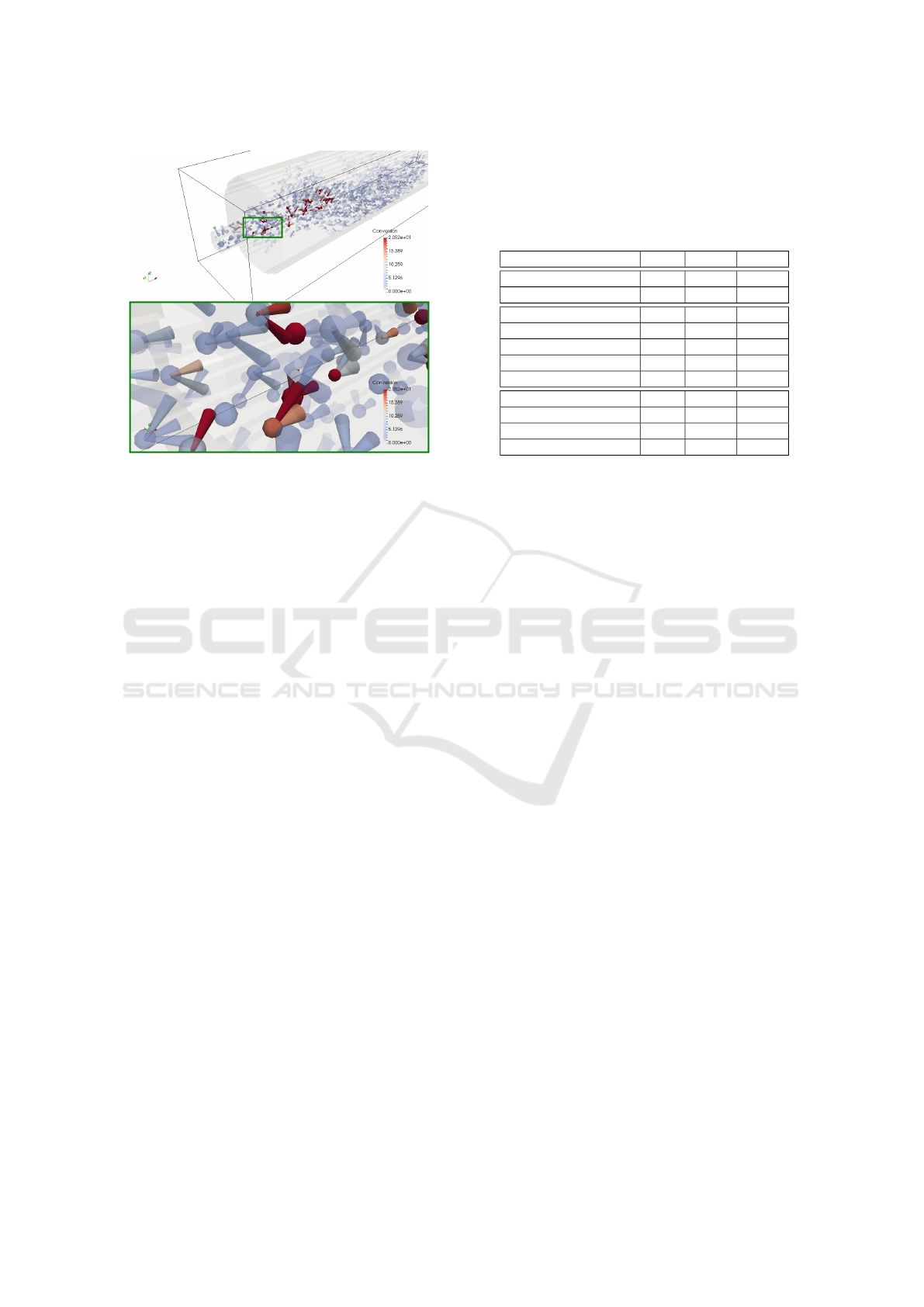
Figure 6: Our energy transport glyphs derived from time
step 49200 → 49800. The outflow from the inner regions of
the nozzle’s jet toward the outer layer can be immediately
derived. Also the energy ’dissipating’ right after exiting the
nozzle is rather low (small cone diameters in glyph) the con-
version is very high (red color).
seen in Fig. 3(a). He appreciated that outflow through
the top boundary condition, accounting for the loss of
energy over the domain, can be extracted from the vi-
sualization. However, the domain scientist identified
this visualization inadequately visualizes the energy
flow behavior around the prominent region of inter-
est, the structure in the fluid flow. This is addressed
in the Glyph Coverage image (Fig. 3(c)), which we
presented as a solution. The scientist really liked
the clear visualization and the easy interpretation of
the glyph, and had no problem extracting informa-
tion about energy flow, when asked about the infor-
mation gained. He also was intrigued about the vol-
ume visualization of the conversion ratio. In sum-
mary, the expert was clearly interested in the visu-
alization, and appreciated the fact that the informa-
tion is easily gained from both visualization types.
He was especially intrigued by the Sparse Rendering
/ Importance-Weighted Glyph Placement variants for
allowing both an option for overview while enabling
a detailed examination for more interesting features.
Overall, he expects the visualization in general to be
very valuable, and will yield a significant improve-
ment for the analysis of flow in general.
6.5 Timings
There are several steps to compute during the exe-
cution of the algorithm. The timings for calculating
the input energy distributions (i.e. the kinetic and in-
ternal energy from state variables) can be neglected
Table 1: Timings for the different steps performed for
preparing the problem and running the minimum cost flow
algorithm. Once the fluxes have been determined, the var-
ious mappings can be generated and manipulated interac-
tively. The relevant section is given in parentheses. Un-
mentioned timings were negligible ( 10ms).
Data elements Beam 5jets nozzle
Number of nodes 28938 573440 211248
Number of edges 319665 6382336 5116252
Process Graph
Normalization (4.3) 0.7 s 3.85 s 1.41 s
Centers (4.4) 1.02 s 18.25 s 14.43 s
Build graph (4.4) 0.42 s 8.49 s 6.55 s
Run solver (4.4) 10.31 s 624.10 s 557.30 s
Generate Mappings
Total Energy (5.2) 0.05 s 0.92 s -
Energy Conversion (5.2) 0.06 s 1.38 s 1.51 s
Weighted Glyphs (5.3) - 2.13 s 2.10 s
( 1s). As the mesh may be unstructured with ar-
bitrary cells, and varying over time (as is the case for
the beam in cross flow), cell centers need to be recom-
puted for each time step, taking the arithmetic mean
of the vertices defining a cell. The normalization of
the total energy to exactly match contained energy be-
tween source and destination time step, as explained
in section 4, is then performed. Next, the nodes and
edges for the minimum cost flow algorithm are allo-
cated and established. When the graph is established
the algorithm can be executed to solve the problem.
Finally, one or more visualization types can be chosen
to be performed on the algorithm’s result. Timings
were taken for all data sets and the individual steps
performed, the results are given in Tab. 1. The tim-
ings are clearly dominated by the minimum cost flow
algorithm, which has a high complexity in the num-
ber of nodes and edges. Once calculated, the various
mappings can be produced interactively. The proto-
type implementation has various ways for improving
performance, in particular using additional physical
constraints like fluid parameters to reduce the number
of edges needed for the solution of the minimum cost
flow problem.
7 CONCLUSION
We presented a technique to visualize the transport of
and conversion between internal and kinetic energy
from arbitrary compressible flow simulations. For this
purpose, we modeled our energy transportation prob-
lem as a graph, and solved it via a minimum cost
flow solver, inherently respecting energy conserva-
tion. Here, we explicitly considered of various sim-
ulation parameters like boundary conditions and en-
IVAPP 2017 - International Conference on Information Visualization Theory and Applications
62

ergy transport mechanisms. Based on the resulting
flux, we then derived a local measure for the conver-
sion between energy forms using the distribution of
internal and kinetic energy. We finally employed dif-
ferent mapping approaches, and evaluated our tech-
nique by means of different simulation data sets and
feedback by a domain scientist. In particular, we in-
troduced glyphs to specifically depict convergence.
By controlling glyph placement via the conversion ra-
tio, we minimized occlusion problems by focusing on
regions that are generally of interest. For future work,
we aim to further study and evaluate our approach
with additional types of simulations, as well as data
from measurements obtained via experiments. An-
other promising improvement to enhance the quality
of the total energy flux estimation, is deriving edge
weights from given physical information, e.g. using
the (easy to calculate) momentum flux to favor certain
edges. For the Importance-Weighted Glyph Place-
ment, glyph density and size could be automatically
adjusted in a view-dependent fashion.
REFERENCES
Bonneel, N., van de Panne, M., Paris, S., and Heidrich, W.
(2011). Displacement interpolation using lagrangian
mass transport. ACM Trans. Graph., 30(6):158:1–
158:12.
Borgo, R., Kehrer, J., Chung, D. H. S., Maguire, E.,
Laramee, R. S., Hauser, H., Ward, M., and Chen, M.
(2013). Glyph-based visualization: Foundations, de-
sign guidelines, techniques and applications. Euro-
graphics Association.
Boring, E. and Pang, A. (1996). Directional flow visual-
ization of vector fields. In Visualization ’96. Proceed-
ings., pages 389–392.
Goedbloed, J. and Poedts, S. (2004). Principles of Magneto-
hydrodynamics: With Applications to Laboratory and
Astrophysical Plasmas. Cambridge University Press.
Goldberg, A. V. and Tarjan, R. E. (1986). A new approach
to the maximum flow problem. In Proceedings of
ACM Symposium on Theory of Computing, STOC ’86,
pages 136–146, New York, NY, USA. ACM.
Goldberg, A. V. and Tarjan, R. E. (1990). Finding
minimum-cost circulations by successive approxima-
tion. Math. Oper. Res., 15(3):430–466.
Hasert, M. (2014). Multi-scale Lattice Boltzmann simu-
lations on distributed octrees; 1. Aufl. PhD thesis,
M
¨
unchen.
Hlawatsch, M., Leube, P., Nowak, W., and Weiskopf,
D. (2011). Flow radar glyphs-static visualization
of unsteady flow with uncertainty. IEEE TVCG,
17(12):1949–1958.
Kraus, M. and Ertl, T. (2001). Interactive data exploration
with customized glyphs. In WSCG, pages 20–23.
Kroes, T., Post, F. H., and Botha, C. P. (2011). Interactive
direct volume rendering with physically-based light-
ing. techreport 2011-11, TU Delft. 1–10.
Landau, L. D. and Lifshitz, E. M. (1987). Fluid Mechanics,
Second Edition. Butterworth-Heinemann, 2 edition.
Laramee, R. S., Schneider, J., and Hauser, H. (2004).
Texture-based flow visualization on isosurfaces from
computational fluid dynamics. In IEEE TVCG / Vis-
Sym, pages 85–90.
Leal, L. G. (2007). Advanced transport phenomena: fluid
mechanics and convective transport processes. Cam-
bridge University Press.
McLoughlin, T., Jones, M. W., Laramee, R. S., Malki, R.,
Masters, I., and Hansen, C. D. (2013). Similarity
measures for enhancing interactive streamline seed-
ing. IEEE TVCG, 19(8):1342–1353.
McLoughlin, T., Laramee, R. S., Peikert, R., Post, F. H., and
Chen, M. (2010). Over two decades of integration-
based, geometric flow visualization. Computer
Graphics Forum, 29(6):1807–1829.
Meyers, J. and Meneveau, C. (2012). Flow visualization
using momentum and energy transport tubes and ap-
plications to turbulent flow in wind farms. J. Fluid
Mech. (2013), vol. 715, pp. 335-358.
Ropinski, T., Oeltze, S., and Preim, B. (2011). Survey
of Glyph-based Visualization Techniques for Spatial
Multivariate Medical Data. Computers & Graphics.
Rubner, Y., Tomasi, C., and Guibas, L. (2000). The earth
mover’s distance as a metric for image retrieval. Inter-
national Journal of Computer Vision, 40(2):99–121.
Sadlo, F.,
¨
Uffinger, M., Pagot, C., Osmari, D., Comba, J.,
Ertl, T., Munz, C.-D., and Weiskopf, D. (2011). Visu-
alization of cell-based higher-order fields. Computing
in Science and Engineering, 13(3):84–91.
Sankey, H. R. (1905). The energy chart : practical appli-
cations to reciprocating steam-engines. Albert Frost
and Sons.
Schroeder, W. J., Volpe, C. R., and Lorensen, W. E. (1991).
The stream polygon-a technique for 3d vector field
visualization. In IEEE Conference on Visualization,
pages 126–132, 417.
Schultz, T. and Kindlmann, G. (2010). A maximum en-
hancing higher-order tensor glyph. Computer Graph-
ics Forum, 29(3):1143–1152.
Tong, X., Zhang, H., Jacobsen, C., Shen, H.-W., and Mc-
Cormick, P. (2016). Crystal Glyph: Visualization of
Directional Distributions Based on the Cube Map. In
EuroVis 2016 - Short Papers.
¨
Uffinger, M., Schweitzer, M. A., Sadlo, F., and Ertl, T.
(2011). Direct visualization of particle-partition of
unity data. In Proceedings of VMV, pages 255–262.
Wittenbrink, C. M., Pang, A. T., and Lodha, S. K. (1996).
Glyphs for visualizing uncertainty in vector fields.
IEEE TVCG, 2(3):266–279.
Transportation-based Visualization of Energy Conversion
63
