Simulation of Radar Signal Processing based on Matlab
Hanwen Wu
(Unit 92941 , Huludao liaoning 125000, China)
Key words: Signal processing; quadrature sampling, pulsed compression; echo accumulation.
Abstract: The simulation of radar signal processing is an important part of the simulation of the radar system. This
paper introduces a method of the simulation of radar signal processing based on Matlab, including the
simulation of radar echo and clutter, and researches the simulation method of important technologies in the
radar signal processing, including quadrature sampling, pulse compression, echo accumulation and CFAR
detector. The work in this paper can overcome the disadvantages such as difficulty and lengthiness and
show the convenience and simplicity of the simulation of radar signal processing based on MATLAB.
1 INTRODUCTION
The modern radar system is getting so complicated
that it can not be processed with simple analytical
methods. Thus people usually make use of
computer to simulate the functions and
performances of the system, which is featured by
great convenience, flexibility and low cost.
However, Matlab has provided a powerful
simulation platform which facilitates the operation
for the simulation of the majority radar system.
The typical radar is made up by antenna,
transmitter, receiver, signal processor, servo
system and terminal unit(Lufei Ding,1984). In the
paper, the authors mainly probe into the radar
signal processing part, and illustrate the application
of Matlab in the radar signal processing system
with the case of a certain pulsed compression radar
signal processing system.
2 GENERATION OF
SIMULATED SIGNAL
2.1 Generation of Radar Signal
The modern radar has diversified systems. The
form of signal can be selected according to the
radar system. In the following part, the method of
how to generate chirp signals in Matlab will be
introduced briefly.
Matlab provides the modulate function which
can generate chirp signals in a convenient manner.
The calling format for the modulate function is
shown as follows:
y = modulate (x, fc,fs, ‘method’,opt)
The parameter x represents the sequence of
modulating signal, fc represents the carrier
frequency, and fs represents the sampling
frequency. The ‘method’ is used to decide which
kind of modulation will be adopted. opt represents
the modulation sensitivity, that is, the stepping
coefficient of chirp signal.
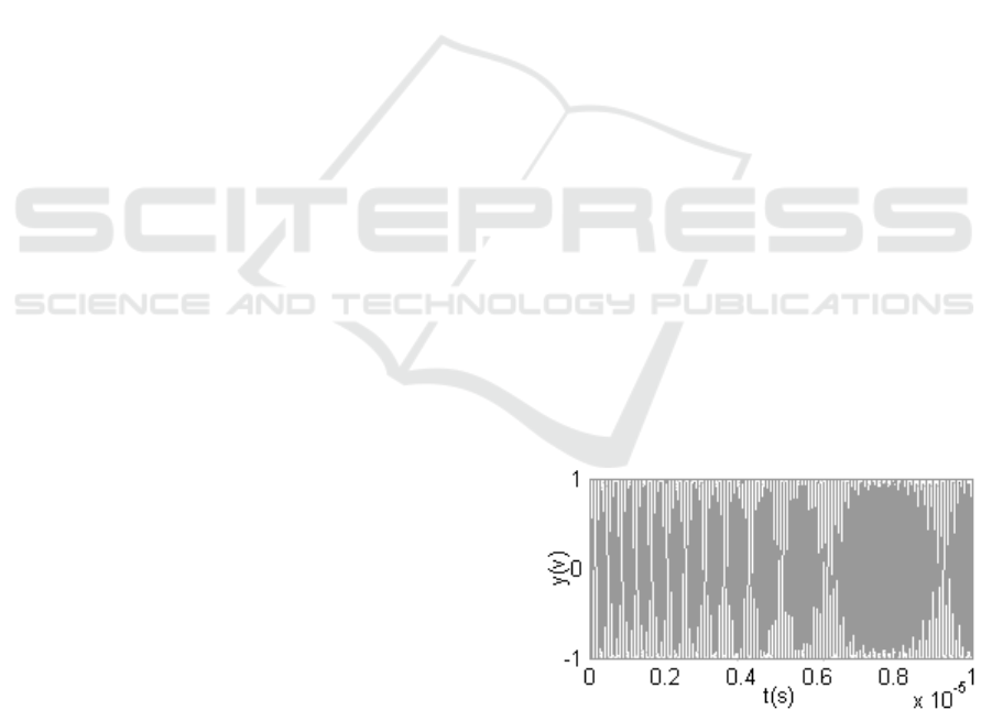
A chirp signal, with the starting frequency of
10MHz, tuning bandwidth of 2MHz, sampling
frequency of 100MHz and pulse bandwidth of
10µs, is generated by a modulate function. The
output result is shown in Figure 1.
Figure 1. Chirp Signal with Carrier Wave of 10MHz and
Bandwidth of 2M
2.2 Generation of Noise and Clutter
In the real radar echo signals, there are not only
signals reflected from targets but also various
299
Wu H.
Simulation of Radar Signal Processing based on Matlab.
DOI: 10.5220/0006449402990304
In ISME 2016 - Information Science and Management Engineering IV (ISME 2016), pages 299-304
ISBN: 978-989-758-208-0
Copyright
c
2016 by SCITEPRESS – Science and Technology Publications, Lda. All rights reserved
299
noises and clutters such as thermal noises from the
receiver, ground clutters, weather clutters and so
on. Noises and clutters can be analyzed only with
statistical properties because neither of them are
deterministic signals. In the following part, the
common method of generating noises and clutters
will be presented.
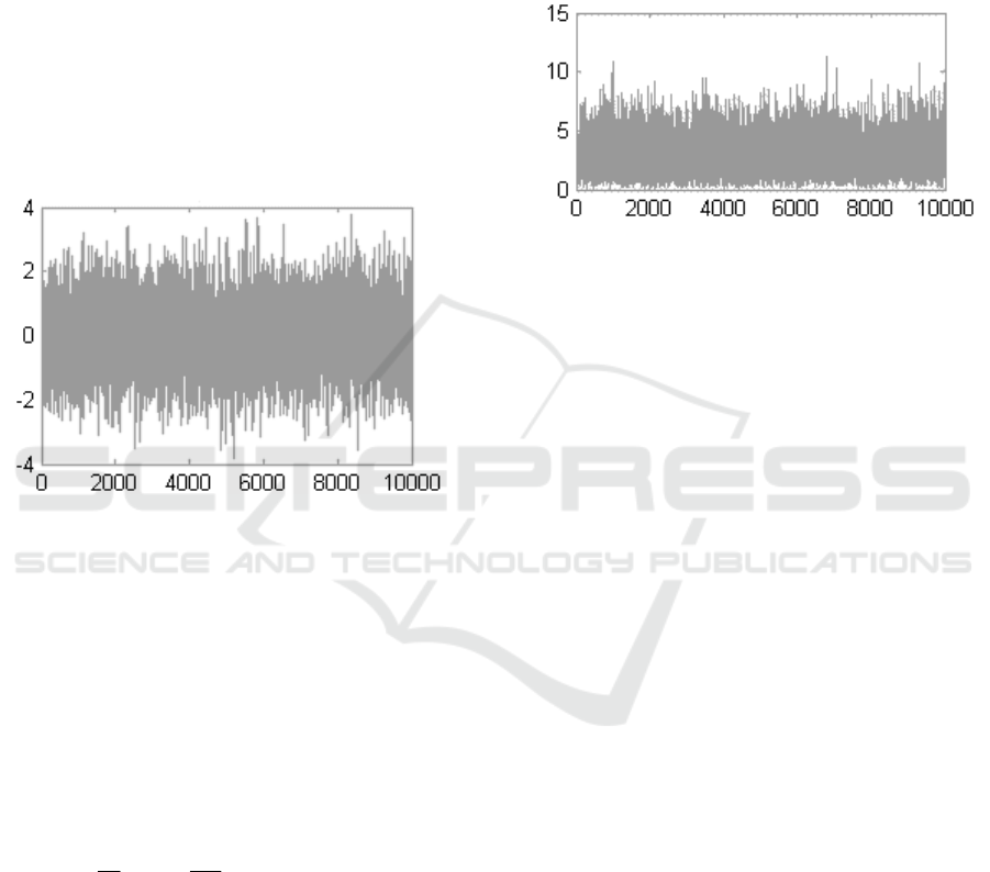
1) Thermal noises subject to Gaussian
distribution (random sequence): Matlab provides
the random function which is used to generate the
random number in standard Gaussian distribution.
random (m,n) can generate the m×n random
sequence matrix. Therefore, a random sequence
subject to Gaussian distribution can be easily
generated by a random function, as shown in
Figure 2.
Figure 2. Random Sequence Subject to Gaussian
Distribution
2) Generation of clutters in Rayleigh
distribution: The Rayleigh distribution is the most
frequently used and the earliest statistical model.
When there are many scatterers within the
discernible range of radar, the envelope amplitude
for synthesizing echo is subject to the Rayleigh
distribution according to the random characteristics
of the amplitude and phase position of scatterers. If
x represents the envelope amplitude of the clutter
echo subject to Rayleigh distribution, then its
probability density function can be expressed as
⎩
⎨
⎧
<
≥−
=
0,0
0),exp(
)(
22
2
x
x
xp
xx
σσ
(1)
In this formula, σ is the standard deviation of
clutter.
Matlab provides a raylrnd function which is
used to generate the random number in Rayleigh
distribution. In the raylrnd (B,m), B is the
parameter of Rayleigh distribution, and m is a
one-dimensional vector that contains two elements
which represent the line number and column
number of the random number matrix which is
subject to Rayleigh distribution respectively.
Generally, the line number is set as 1, and the
column number corresponds to the duration of
clutter. When the parameter of Rayleigh
distribution σ=2, the clutter generated with the
raylrnd function is shown as Figure 3.
Figure 3. Clutter in Rayleigh Distribution
3 SIMULATION OF SIGNAL
PROCESSING SYSTEM
The purpose of processing radar signals is to
remove the unwanted signals (such as clutter) and
the interference, and to extract and intensify the
echo signals generated by the target. The radar
signal processing provides many functions, and
functions of different radars also vary(You
He,1999). In this paper, a certain pulse
compression radar’s signal processing part is
simulated. The signal processing part of a typical
pulse compression radar mainly has the functions
of A/D sampling, quadrature demodulation, pulse
compression, video integration, constant false
alarm processing and so on. Hence, the simulation
model for the pulse compression radar’s signal
processing is as shown in Figure 4.
3.1 Quadrature Demodulation
Module
Before the pulse compression for radar ’ s
intermediate-frequency signals, it is necessary to
transform these signals into the I and Q quadrature
signals with the zero intermediate frequency.
The intermediate-frequency signals can be
expressed as
ISME 2016 - Information Science and Management Engineering IV
300
ISME 2016 - International Conference on Information System and Management Engineering
300
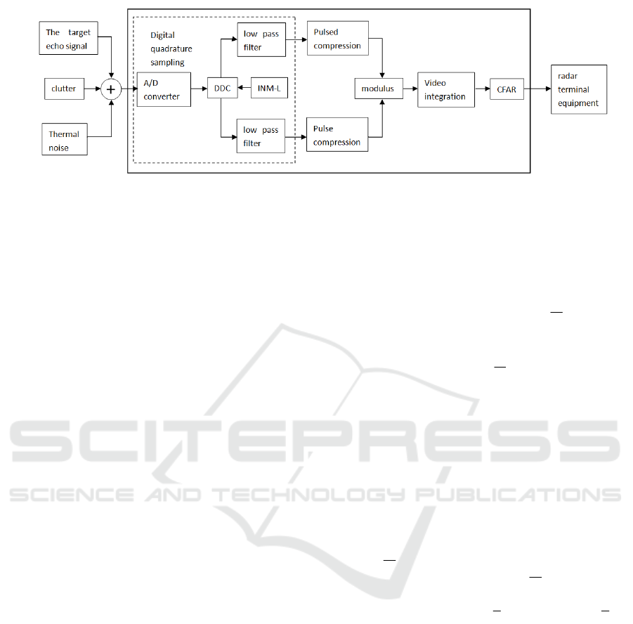
Figure 4. Simulation Model for Pulse Compression Radar’s Signal Processing
))(2cos()()(
0
ttftAtf
IF
φ
π
+
= (2)
In the formula, f
0
is the carrier frequency.
To set
⎩
⎨
⎧
=
=
)(sin)()(
)(cos)()(
ttATQ
ttATI
φ
φ
(3)
Then
tftQtftItf
IF 00
2sin)(2cos)()(
π
π
−
= (4)
In the simulation, all the signals are expressed as
discrete time series. Set the sampling period as T,
and then the intermediate-frequency signal will be
fIF (rT). Similarly, the local oscillating signals,
after being sampled, will be expressed as
)exp(
0
rTjf
local
ω
−= (5)
The digitized intermediate-frequency signals and
local oscillating signals will turn into baseband
signals after they are multiplied and demodulated
and then pass the low-pass filter. The baseband
signal fBB (r) can be expressed as
{}
1
0
0
() ( )cos( ) ()
N
BB IF
n
f
r f rn rn Thn
ω
−
=
=−− −
∑
{}
1
0
0
()sin() ()
N
IF
n
j
frn rn Thn
ω
−
=
−−
∑
(6)
Wherein, h(n) is the pulse response of the
low-pass filter which has an accumulated length of
N.
According to the practical application, the
sampling using Nyquist sampling rate only will not
obtain good mixing signals and filtering results.
Generally, good real part and imaginary part of
signal can be obtained when the sampling
frequency fs is four times of the center
frequency(Yingle Fan,2001). When the sampling
frequency fs=4f
0
, and 2/
0
π
ω
=T , the baseband
signal can be simplified as
1
0
() ( )cos( ) ()
2
N
BB IF
n
f
r
f
rn rn hn
π
−
=
⎧⎫
=
−− −
⎨⎬
⎩⎭
∑
1
0
()sin() ()
2
N
IF
n
j
frn rn hn
π
−
=
⎧⎫
−−
⎨⎬
⎩⎭
∑
(7)
The steps for simulation of quadrature
demodulation using Matlab are shown as follows.
1) To generate the ideal chirp signal y;
2) To generate the I-channel local oscillating
signal and the Q-channel local oscillating signal.
Set f
0
as the center frequency of the local
oscillating signal, f
s
as the sampling frequency, n as
the length of the chirp signal’s time series, then the
I-channel local oscillating signal will be
)2cos(
0
π
s
f
f
n . Likewise, the Q-channel local
oscillating signal will be
)2sin(
0
π
s
f
f
n . When f
s
=4f
0
, the I-channel and Q-channel local oscillating
signals will be
)cos(
2
π
n
and )sin(
2
π
n
respectively.
3) Multiplying the chirp signal y by the double
local oscillating signal to obtain the I-channel
signal and the Q-channel signal.
4) The I-channel signal and the Q-channel signal
pass through the low-pass filter and filter off the
high-frequency component in order to get the final
result of demodulation(Haimang Hu,2004). Matlab
provides a convenient filter function filter(b,a,x),
in which x represents the input signal, and b and a
represent the coefficient vectors of the filter
transfer function’s numerator and denominator.
Figure 5 shows the simulation of chirp signal
with Matlab. Figure 6 and 7 show the demodulated
I-channel signal and Q-channel signal respectively.
Simulation of Radar Signal Processing based on Matlab
301
Simulation of Radar Signal Processing based on Matlab
301
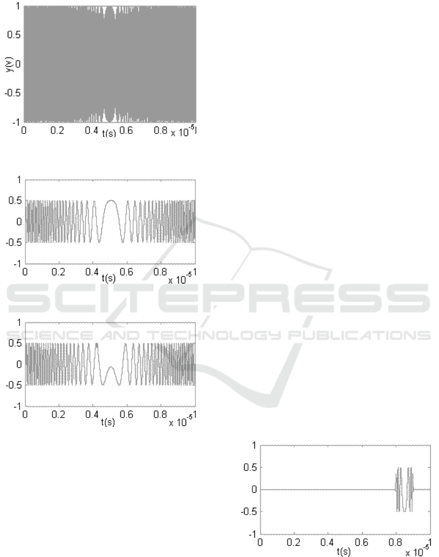
Figure 5. Chirp Signal With the Carrier of 10MHz and
Bandwidth of 2MHz
Figure 6. I-channel Signal after Demodulating the Chirp
Signal
Figure 7. Q-channel Signal after Demodulating the Chirp
Signal
3.2 Pulse Compression Module
Before the pulse compression, it is necessary to
find a matched filter for signals transmitted by
radar(Yu Zhou,2004). In real projects, pulse
compression is usually done in the frequency
domain because it can improve the computation
speed by making use of the FFT algorithm. The
result of pulse compression can be obtained after
multiplying the radar echo by the matched filter’s
frequency domain response and then getting them
transformed with IFFT. Hence, convolution
processing has been replaced, thus greatly reducing
the amount of operation. Therefore, it is necessary
to firstly obtain the matched filter or pulse
compression coefficient for the pulse compression
when simulating the pulse compression. It is easy
to work out the chirp signal’s pulse compression
coefficient, which can be achieved by conjugating
and overturning the ideal chirp signal.
The steps for simulation of chirp signal’s pulse
compression using Matlab are shown as follows.
1) To generate the ideal chirp signal y;
2) To make quadrature demodulation for signals
in order to obtain the demodulated signals ;
3) To generate the ideal chirp compression
coefficient. To achieve this, you shall firstly find
out the matched filter for the signal fbb which has
been processed with quadrature demodulation, and
then work out the pulse compression coefficient by
making use of the discrete Fourier transform.
4) To generate the ideal echo signal and to
process the signal with quadrature demodulation.
The idea echo signal is the echo signal received by
radar within a pulse repetition period, and the
target is assumed to be a stationary-point target.
5) To make pulse compression. Firstly, make the
discrete Fourier transform for the echo signal in
order to obtain signal_fft, and then multiply the
signal_fft and the matched filter’s frequency
domain response, and then make inverse discrete
Fourier transform for it, thus obtaining the result of
pulse compression(Zewei Wang,2005). Assuming
the signals transmitted by radar are the chirp
signals, the relevant parameters are shown as
follows: bandwidth 10µs, center frequency 10MHz
and tuning bandwidth 2MHz. The frequency of
sampling radar’s echo signals is 40MHz. The
intermediate frequency is processed with
quadrature down-conversion. In Figure 8 and 9, the
oscillograms have shown the simulation of radar
pulse compression using Matlab.
Figure 8. Result Obtained after the Quadrature
Demodulation for Echo Signal
ISME 2016 - Information Science and Management Engineering IV
302
ISME 2016 - International Conference on Information System and Management Engineering
302
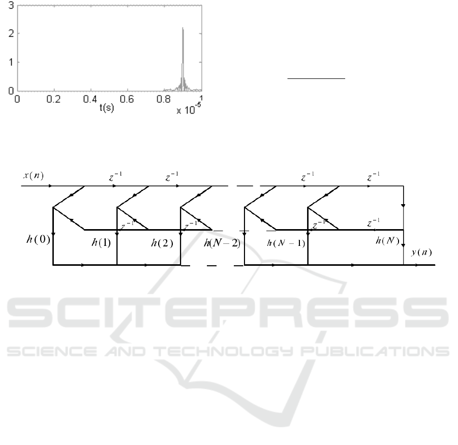
Figure 9. Result Obtained after the Pulse Compression
for Echo Signal
3.3 Echo Accumulation Module
The modern radars make detection based on
multi-pulse observation(). The integration of
multiple pulses can effectively improve the
4
sin ( )
()
na
hn
na
θ
θ
Δ
=
Δ
(9)
Δθ represents the angle that the antenna has
swept across within a pulse repetition period. Such
integration can be realized by the FIR integrator,
with its structure shown in Figure 10.
Figure 10. Structural Diagram for FIR Accumulator
3.4 Constant False Alarm Rate
(CFAR) Processing Module
There are many methods to make constant false
alarm processing. In broad classification, there are
mean level CFAR, order statistics CFAR, clutter
map CFAR and so on. There are many ways to
realize the mean level CFAR, including cell
averaging, GO, SO and so on, all of which operate
under the same fundamental theory. The
procedures for simulation of CFAR using Matlab
are shown as follows.
1) To generate the point-target echo which has
superimposed the Rayleigh clutter and thermal
noise. In this step, the Gaussian thermal noise and
Rayleigh clutter are generated with the
above-mentioned method, and then are
superimposed with the point-target echo, during
which the amplitudes of Rayleigh clutter and
thermal noise shall be weighted.
2) To make constant false alarm processing for
the point-target echo which has superimposed
Rayleigh clutter and thermal noise. In this step, the
number of reference cells shall be determined
firstly. If the number of reference cells are 16, the
mean value of the first point noise for constant
false alarm processing will be decided by its
subsequent 16 points of noises, while mean value
of the noises from the second point to the 16
th
point will be jointly decided by the 16 points of
noises before and after it. The mean value of noises
on normal data points for constant false alarm
processing is determined by its former 16 points of
noises and its subsequent 16 noises, and the
constant false alarm processing for the last 16
points of noises is the same as that for the first 16
points of noises. The signal output lastly is the
ratio between the estimated mean values of each
detection unit and the clutter.
In the following part, we will simulate the
GO-CFAR using Matlab. The number of reference
cell is 16, and the radar’s pulse repetition period is
1ms. There are clutter echoes subject to Rayleigh
distribution in the range from 7.5 km to 30 km
away, and there is a point target 15km away. The
results of simulation are shown in Figure 11 and
Figure 12.
Simulation of Radar Signal Processing based on Matlab
303
Simulation of Radar Signal Processing based on Matlab
303
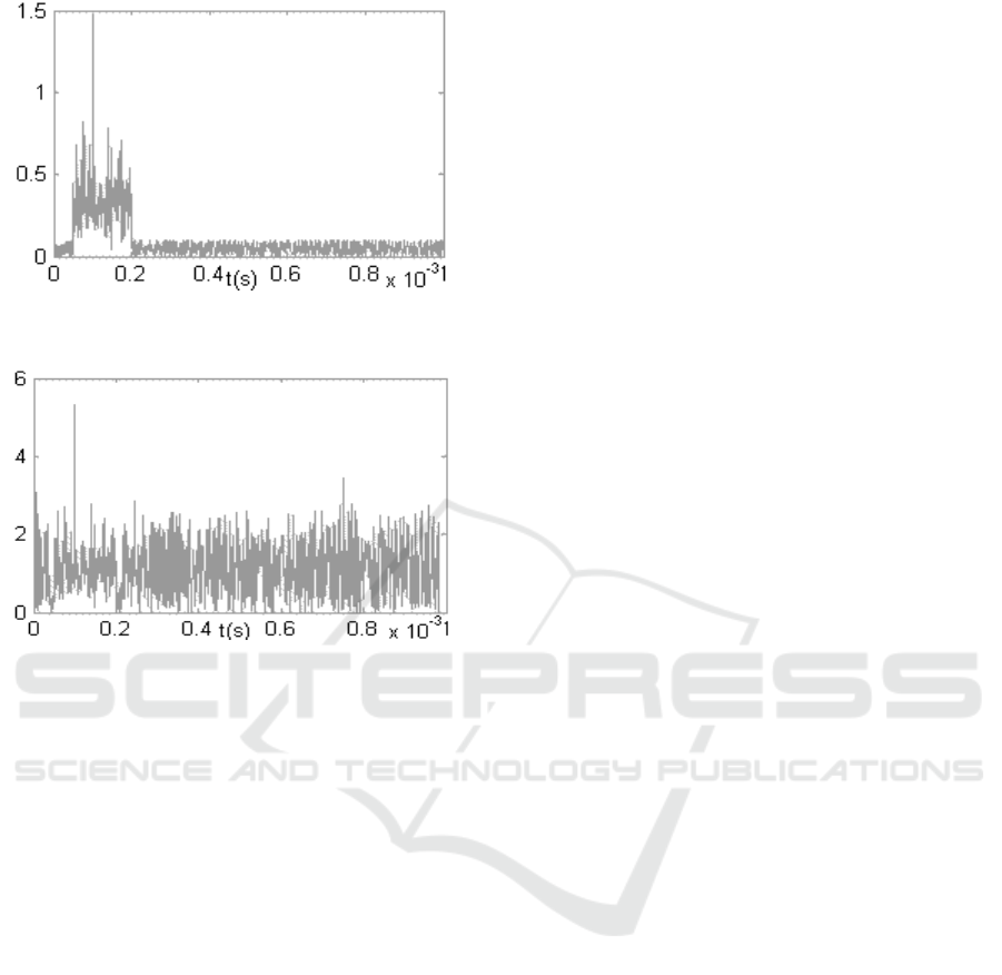
Figure 11. Target Echoes Which Have Superimposed
Clutters in Rayleigh Distribution and Thermal Noise
Figure 12. Outcome of GO-CFAR
4 CONCLUSIONS
In the simulation of radar signal processing system
using Matlab, a system model can be formed
rapidly, and your design concept can be reflected
in each little detail. It is featured by a short
modeling time and a high calculation accuracy.
The model formed is simple and clear. The model
and evaluation result can be revised, and the
system behavior can be verified at any phase of the
design. In this paper, the authors have take a
certain pulse compression radar as an example to
study the Matlab-based simulation of radar signal
processing, which achieves good outcome.
REFERENCES
Lufei Ding and Ping Zhang, 1984.Radar System. Xi’an:
Xidian University Press
You He, Jian Guan et al,1999.Radar Automatic
Detection and Constant False Alarm Processing.
Beijing: Tsinghua University Press.
Yingle Fan, 2001.Detailed Introduction of Application of
MATLAB-based Simulation. Beijing: Posts and
Telecom Press.
Yu Zhou, Linrang Zhang and Hui Tian, 2004. Radar
System Simulation Based on Matlab/ Simulink [J].
Computer Simulation.
Haimang Hu and Wanhai Yang, 2004. Simulink-based
Modeling and Simulation for Pulse Compression
Radar . Radar and Countermeasures.
Zewei Wang and Hongjin Jia,2005. Research on
Modeling and Simulation of Search Radar Radar and
Countermeasures.
ISME 2016 - Information Science and Management Engineering IV
304
ISME 2016 - International Conference on Information System and Management Engineering
304
