Bathymetric Mapping of Shallow Rivers with

UAV Hyperspectral Data

Valeria Gentile

1,2

, Marek Mrόz

, Marie Spitoni

, Jérôme Lejot

, Hervé Piégay

and Luca Demarchi

Dept. of Information, Electronics & Telecom. Eng. (DIET), Univ. of Rome “Sapienza”, via Eudossiana 18, Rome, Italy

Université de Lyon, UMR 5600 EVS, Ecole Normale Supérieure, Lyon Cedex 07, France

Dept. of Photogrammetry & Remote Sensing, Univ. of Warmia and Mazury in Olsztyn, ul. Oczapowskiego, Olsztyn, Poland

Université de Lyon, UMR 5600 EVS, Université Lumière Lyon 2, Campus Porte des Alpes, Bron Cedex, France

WarsawUniversity of Life Sciences Nowoursynowska 166, 02-787 Warsaw, Poland

valeria.gentile@uniroma1.it, {valeria.gentile, marie.spitoni, herve.piegay}@ens-lyon.fr,

marek.mroz@uwm.edu.pl, jerome.lejot@univ-lyon2.fr, demarchi.luca.ld@gmail.com

Keywords: Bathymetry, High spatial resolution, Hyperspectral images, Fluvial morphology, Remote sensing.

Abstract: Airborne images have long been used to support environmental monitoring due to their synoptic capability

to cover wide areas with high spatial and temporal resolution. The potential for bathymetric mapping by

airborne remote sensing has been addressed and demonstrated in several studies by means of imaging and

non-imaging techniques. In this paper we evaluate the potential to retrieve water depth of shallow river from

high resolution hyperspectral images using an empirical model, applicable under a range of specific field

conditions and in a definite interval of wavelengths.

1 INTRODUCTION

The necessity to preserve water resources and

ecosystems has led to an increasing interest in

monitoring the morphological status of water bodies.

Through a constant data collection on the long term,

it is possible to determine trends in monitored

parameters and to decide suitable strategies in order

to prevent river channel degradation or to restore its

original status.

Remote Sensing (RS) has long been used to

support environmental monitoring of fluvial

environments due to its synoptic capability to cover

wide areas with high spatial and temporal resolution

and to detect features that are not rapidly and easily

evaluable with in situ measurements. Remote

sensing techniques have been also widely applied to

assess bathymetry of water body (Carbonneau, Lane

and Bergeron, 2006, Fonstad and Marcus, 2005,

Lane, Westaway and Murray Hicks, 2003), being the

only effective alternative to measurements collected

by echo sounder mounted on boat, in very shallow

and braided rivers, impossible to be entirely

navigated. Furthermore ground surveys are

extremely time-consuming, require a consistent

deployment of manpower and provide a low spatial

sampling of acquired data despite to their accuracy.

As reviewed by Feurer, Bailly, Puech, Le Coarer

and Viau (2008), besides echo sounder and GPR

(Ground Penetrating Radar), both requiring ground

surveys, three remote sensing approaches exist for

mapping water depth through imaging and non

imaging techniques (Gao, 2009). These are spectral

methods, photogrammetry and bathymetric LIDAR

(Light Detection and Ranging). Spectral methods

exploit the attenuation of electromagnetic wave

through the water interface in order to derive water

depth. Their capability for mapping bathymetry has

been addressed in several studies, using data

acquired in the visible spectrum from UAV

platforms (Lejot et al., 2007, Feurer et al., 2008) or

Airborne Thematic Mapper data simulated from

ground based measurements collected through

spectroradiometer (Gilvear, Hunter ad Higgings

2007) or AISA (Airborne Imaging Spectrometer for

Applications) data (Legleiter, Roberts and

Lawrence, 2009).

Gentile V., MrÏ

Nz M., Spitoni M., Lejot J., PiÃl’gay H. and Demarchi L.

Bathymetric Mapping of Shallow Rivers with UAV Hyperspectral Data.

DOI: 10.5220/0006227000430049

In Proceedings of the Fifth International Conference on Telecommunications and Remote Sensing (ICTRS 2016), pages 43-49

ISBN: 978-989-758-200-4

In our study we evaluate the potential to retrieve

water depth of shallow river from very high

resolution hyperspectral images, using a simple

empirical model, applicable under a range of

specific field conditions. In doing so, we take

advantages first from the capability of UAV

platforms to acquire very high resolution images,

combined with the possibility given by hyperspectral

sensors to investigate the model behaviour over a

wide range of wavelengths in addition to the visible

spectrum.

In our paper we provide a detailed description of

the study site in section 2. In section 3 is explained

the overall process to obtain the final results: the

acquisition campaign with used sensors and platform

is described in subsection 3.1, in subsection 3.2 the

entire processing chain to derive the final

orthomosaics from raw hyperspectral data cubes is

illustrated, in subsection 3.3 the physical model

adopted to derive the relation between the

radiometric pixel value and the water depth is

explained. In subsection 3.4 processing applied to

the final orthomosaics to establish the goodness of

the relation previously described is explained.

Results and conclusion follow in sections 4 and 5

respectively.

2 STUDY SITE

The acquisition campaign was carried out along a

channel reach of the Ain River in the south-east part

of France. The Ain River drains a watershed surface

of about 3700 km² along 200 km. It rises in the Jura

Mountains, then it flows through a steep

mountainous relief, before reaching its Lower Valley

(Liébault and Piégay, 2002). The river in its Lower

Valley flows through 50 km, in alluvial deposits

(Bravard, 1986) where it is free to laterally and

vertically adjust. Its depth ranges between 0 to 5 m

(Lejot et al., 2007). Its hydrology is dominated by

snowmelt mixed with rainfall. The mean annual

discharge is 120 m

-1

, ranging between 17 m

-1

1600 m

-1

(1-in-50 year flood) at Pont d’Ain and

Chazey-sur-Ain gauging stations according to the

banque HYDRO (http://www.hydro.eaufrance.fr/). A

chain of 5 main hydroelectric dams were built until

the 70's in its middle V-shape valley section. These

dams have undergone important changes in the

Lower Valley, e.g. reduction of peak flows and

channel narrowing or degradation (Liébault and

Piégay, 2002).

The study site (Figure 1), approximately 700 m

long, between Pont d’Ain and Priay, is located in the

Ain Lower Valley, northeast of the city of Lyon. It

was chosen because of its fairly morphological and

channel stability (paved riverbed and low lateral

mobility). Due to the lack of in situ water depth data

synchronous with imagery data, we used the

simulated hydrological parameters from the

numerical model developed by Paquier, Camenen,

Le Coz and Béraud (2014). This model runs over

ADCP and GPS cross-sectional surveys performed

in 2013 and 2014 (Naudet, Le Coz, Camenen and

Paquier, 2015). Riverbed changes were assumed to

be negligible on the study reach since the last 3

years (the mean absolute error for the modelled 2013

water level elevation is 15 cm).

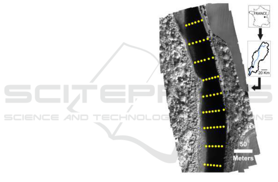
Figure 1: Orthomosaic at the central wavelength λ=776nm

and geographical location of the study site; in yellow

sampling points of 2D hydraulic model.

3 METHODS

3.1 Data Collection

The study area was imaged twice on 28

September

2015 in the interval 12h00-12h54 (CEST) using two

coupled cameras mounted on the UAV md4-1000

quadrocopter (table 1):

 digital RGB OLYMPUS EP-2 camera

Fifth International Conference on Telecommunications and Remote Sensing

 Rikola 2D spectral sensor (Makelainen, Saari,

Hippi, Sarkeala and Soukkamaki, 2013).

The Rikola 2D imaging system is a VNIR sensor

based on the Piezo-Actuated Fabry-Perot

Interferometer (FPI), working in the spectral range

500 nm - 900 nm. This allows the user to select the

central wavelengths of the bands to be recorded by

setting up the appropriate “air gaps” in the

interferometer. The CCD/CMOS matrix consists of

1024x1024 detectors. Each sensing element has the

size of 5.5x5.5 μm. The camera is characterized by

FOV=37°, focal length f=9mm and F-number=2.8.

The ADC (analog-to-digital converter) is operating

in 12 bit mode. The system is equipped with GPS

receiver and hemispherical irradiance sensor. The

described camera model and software version permit

to acquire 16 bands in full-frame mode or 24 bands

in the half-frame mode (1024x648 pixels) for one

“hypercube” (single frame). The user can also

choose one of the two FWHMs (full width at half

maximum): narrow or wide. The precise values of

the FWHM for each band are determined by the

interferometer itself.

Table 1: Set of spectral bands recorded in the experiment.

First flight – Full frame

mode

Second flight – half frame

mode

Band no.

Central

wavelength

[nm]

FWHM

[nm]

Band no.

Central

wavelength

[nm]

FWHM

[nm]

500

523

516

546

532

569

548

591

564

614

580

643

596

661

612

684

628

707

644

730

676

753

692

776

708

799

724

822

740

845

The pictures were taken at the altitude

MHOG=100 m (mean height over ground) forming

regular blocks of strips with the end lap of 70% and

side lap of 30% for hyperspectral images. The mean

ground resolution of Rikola images was about 6 cm.

The Rikola camera takes the hypercubes with a

constant time interval Δt which was set in our

experiment at 5 s.

For each block of RGB images the overlapping

was bigger (80% and 40% respectively) and the

ground sampling distance (GSD) was about 2 cm.

The number of acquired hypercubes was bigger than

100 for each of two flights, and about 66 of RGB

pictures.

3.2 Data Pre-processing

Acquired RGB images underwent orthorectification

process with Agisoft Photoscan Professional

software. The process consisted of digital

aerotriangulation, image matching, 3D cloud point

and Digital Surface Model generation and the final

ortho-correction. The final RGB orthophotomap had

pixel size 5x5 cm and it was considered as a

background supporting the geometric processing of

acquired hyperspectral data.

The exposition time for Rikola camera is usually

set between 10 and 25 ms depending on sunlight

intensity. In our experiment the exposition was set at

15 ms. Such a value is suitable for taking non-

blurred pictures from moving platform but the

technology of image formation and recording on the

memory card leads to the situation where every band

of the given hypercube has a slightly different

position and external orientation. In these

circumstances there are two alternative ways for

further geometric processing:

 to adjust all bands of the hypercube to a

common frame first and to produce in the next

step all spectral orthomosaics in one

photogrammetric run;

 to split all bands of each hypercube and to

process all frames taken at the same

wavelength in separated photogrammetric

runs forming a set of independent spectral

mosaics.

We adopted the second way because the

automatic geometric adjustment/matching of the

bands taken in visible and infrared spectrum is very

problematic for the scenes without structural points.

Therefore hyperspectral frames were processed

similarly like RGB photos giving as a result a set of

monochromatic orthophotomaps at the resolution of

10 cm with, unfortunately, slightly different

georeferencing. The last step in geometric

processing was the adjustment of all spectral

orthophotomaps to the common frame by affine

transformation based on RGB orthophotomap.

Bathymetric Mapping of Shallow Rivers with

UAV Hyperspectral Data

Prior to the orthorectification at each spectral

band, the radiometric processing needed to be

performed. The first step was the radiometric

calibration of each hypercube to remove the

influence of the black current from measured

signals. The second step was the radiometric

normalization i.e. comparison of the recorded

spectral luminance for each band with the luminance

of the white standardized target. In our case the

Zenith Lite

panel 50x50 cm covered by BaSO4-

based white paint was used. No other atmospheric or

radiometric corrections were applied. Some spectral

bands from second Rikola dataset taken in half-

frame mode were eliminated due to the encountered

errors in pictures recording.

3.3 Bathymetric Model

The spectral radiance observed at the remote sensor

detector L

(λ) for any wavelength λ is expressed as

the sum of four components (Legleiter et al., 2009):

(λ) = L

(λ) + L

(λ)

(1)

where L

(λ) is the radiance reflected from bottom,

(λ) is the radiance from water column, L

(λ) is the

radiance reflected from water surface and L

(λ) is

the path radiance from the atmosphere. Under the

conditions of homogeneous water properties,

shallow river, opportune viewing geometry, low

acquisition altitude, favourable atmospheric

conditions, highly reflective and homogeneous

streambed and relatively clear water, we can

consider negligible the radiance components L

(λ),

(λ), L

(λ) (Legleiter et al., 2009):

(λ) ≈ L

(λ)

(2)

where L

(λ) is (Philpot, 1989, Legleiter et al., 2009):

(λ)=E

(λ)C(λ)T(λ)(R

(λ)-R

(λ))exp(-k(λ)d)

(3)

(λ) is the downwelling solar irradiance, C(λ) is

a constant for transmission across air water

interface, T(λ) is the transmittance of atmosphere,

(λ) is the reflectance of river bottom, R

(λ) is the

volume reflectance of water column, k(λ) is an

attenuation coefficient that accounts for absorption

and scattering of light within the water column

(Maritorena, Morel, Gentili, 1994, Legleiter et Al.,

2009), d is the water depth. Solving with respect to

water depth, we obtain:

ln(L

)=ln(E

CT(R

-R

))-kd

(4)

where we have not considered the dependence on λ

to simplify the notation. The relation (4) suggests

that under the above-mentioned acquisition

conditions and for certain wavelengths, a relation

between the remotely sensed variable L

and the

water depth can be derived and used for mapping

river bathymetry. Replacing L

with the

corresponding value of digital number registered by

the sensor and opportunely calibrated, after several

adjustments we can rewrite (4) as a linear relation

between the natural logarithm of pixel values in the

image and the corresponding values of water depth:

i,j

= a

0,k

1,k

lnP

i,j,k

(5)

where d

i,j

is the water depth in correspondence of

pixel i,j in the image, a

0,k

and a

1,k

are the coefficients

of linear relation related to k-th spectral band and

i,j,k

is the value of pixel i,j at k-th spectral band.

3.4 Data Processing

Before deriving coefficients a

0,k

and a

1,k

of linear

relation (5) for each orthomosaic, through a linear

regression, a median filter with a window of 5x5

was applied to remove residual noise after images

pre-processing.

For each spectral band, the pixel values were

extrapolated from orthomosaics, in correspondence

of the geographical coordinates of bathymetric

values given by the numerical model of Paquier et

al. (2014) applied to the Ain River (Naudet,

Camenen, Le Coz, Paquier and Piégay, 2014). This

2D hydraulic model provides the riverbed elevation,

the water level elevation and the water depth, based

on topographic cross-sections surveyed every 50 m,

increased to every 25 m where the riverbed

geometry rapidly changes.

The coefficients of the linear regression of the

empirical model were calculated with 70% of the

samples randomly extracted from the set of samples

derived in the previous step. The remaining 30% of

samples were used to assess the validity of the

model.

This method was repeated for each orthomosaic

at each spectral band. The goodness of fitting was

assessed by means of the coefficient of

determination calculated on the 70% of samples and

mean absolute error computed on the remaining 30%

of samples.

Fifth International Conference on Telecommunications and Remote Sensing

4 RESULTS

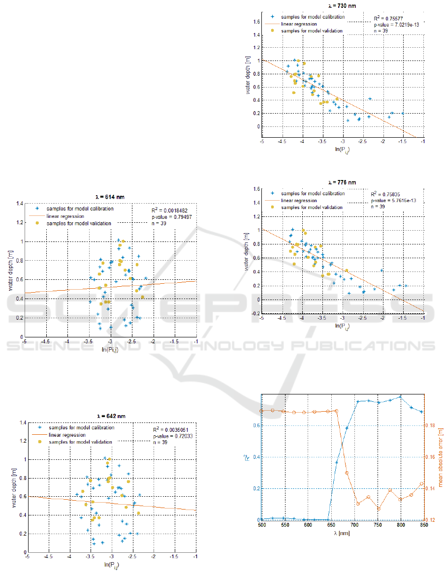
In Figures 2, 3, 4 and 5 a subset of results from the

first survey is shown. The sign of linear regression

slope changes from positive to negative values, as

wavelength increases. This behaviour is due to the

weak correlation between water depth values and

pixel values in the relation (5) at shorter

wavelengths, that increases at longer wavelengths

(Red and Near Infrared), when the absorption due to

water column becomes stronger compared to

reflectance. The increasing trend of correlation

versus wavelength is more evident in Figure 6 where

the coefficient of determination R

and the mean

absolute error with respect to spectral band are

shown.

Figure 2: Linear regression at λ = 614 nm.

Figure 3: Linear regression at λ = 642 nm.

Figure 4: Linear regression at λ = 730 nm.

Figure 5: Linear regression at λ = 776 nm.

The best correlations are obtained in the spectral

range from 700 nm to 800 nm.

Figure 6: Trend of coefficient of determination and mean

absolute error versus wavelength.

In Figures 7, 8, 9 and 10, a subset of results from

the second survey is shown. In Figure 11 trends of

coefficient of determination and mean absolute error

with respect to spectral band are shown, confirming

Bathymetric Mapping of Shallow Rivers with

UAV Hyperspectral Data

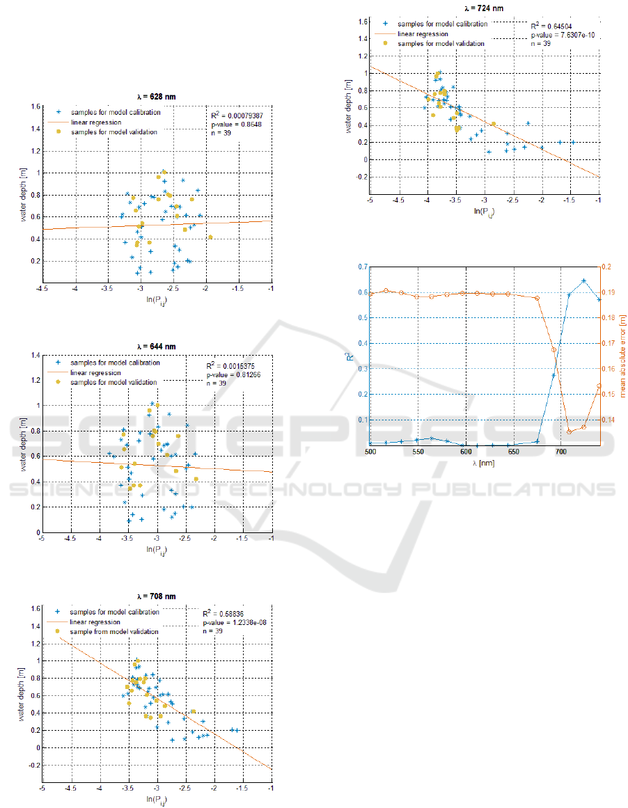
both the best values of correlation in the spectral

range from 700 nm to 750 nm and the increase of

correlation versus wavelength, obtained in the first

survey.

Figure 7: Linear regression at λ = 628 nm.

Figure 8: Linear regression at λ = 644 nm.

Figure 9: Linear regression at λ = 708 nm.

Figure 10: Linear regression at λ = 724 nm.

Figure 11: Trend of coefficient of determination and mean

absolute error versus wavelength.

5 CONCLUSIONS

The results show the potential of UAV hyperspectral

data for bathymetric mapping at centimetre

resolution. The empirical model fits well the water

depth values derived from the hydraulic model in the

spectral range from 700 nm to 800 nm with an

average error less than 0.13 m in the best case when

the water depth ranges from 0.09 m to 1.01 m.

In further studies we intend to apply the

proposed methodology over imagery acquired on

other longer reaches of the Ain River with a wider

range of water depth in order to confirm the model

behaviour with respect to wavelength, to investigate

its applicability over a range of wider environmental

conditions, such as changes in river bottom

morphology and composition, concentration in

suspended sediment, water deepness and finally to

examine obtained results on the basis of sensor

Fifth International Conference on Telecommunications and Remote Sensing

configuration and acquisition mode as pixel ground

resolution and bandwidth.

REFERENCES

Bravard, J. P. (1986). La basse vallée de l'Ain: dynamique

fluviale appliquée à l'écologie. Recherches

Interdisciplinaires sur les Ecosystémes de la Basse-

Plaine de l’Ain: Potentialitees Evolutives et Gestion.

Doc. Cartogr. Ecol, 29, 17-43.

Carbonneau, P. E., Lane, S. N., & Bergeron, N. (2006).

Feature based image processing methods applied to

bathymetric measurements from airborne remote

sensing in fluvial environments. Earth Surface

Processes and Landforms, 31(11), 1413-1423.

Feurer, D., Bailly, J. S., Puech, C., Le Coarer, Y., & Viau,

A. (2008). Very-high-resolution mapping of river-

immersed topography by remote sensing. Progress in

Physical Geography, 32(4), 403-419.

Fonstad, M. A., & Marcus, W. A. (2005). Remote sensing

of stream depths with hydraulically assisted

bathymetry (HAB) models. Geomorphology, 72(1),

320-339.

Gao, J. (2009). Bathymetric mapping by means of remote

sensing: methods, accuracy and limitations. Progress

in Physical Geography, 33(1), 103-116.

Gilvear, D., Hunter, P., & Higgins, T. (2007). An

experimental approach to the measurement of the

effects of water depth and substrate on optical and

near infra-red reflectance: A field-based assessment of

the feasibility of mapping submerged instream habitat.

International Journal of Remote Sensing, 28(10),

2241-2256.

Lane, S. N., Westaway, R. M., & Murray Hicks, D.

(2003). Estimation of erosion and deposition volumes

in a large, gravel‐bed, braided river using synoptic

remote sensing. Earth Surface Processes and

Landforms, 28(3), 249-271.

Lejot, J., Delacourt, C., Piégay, H., Fournier, T., Trémélo,

M. L., & Allemand, P. (2007). Very high spatial

resolution imagery for channel bathymetry and

topography from an unmanned mapping controlled

platform. Earth Surface Processes and Landforms,

32(11), 1705-1725.

Legleiter, C. J., Roberts, D. A., & Lawrence, R. L. (2009).

Spectrally based remote sensing of river bathymetry.

Earth Surface Processes and Landforms, 34(8), 1039-

1059.

Liébault, F., & Piégay, H. (2001). Assessment of channel

changes due to long-term bedload supply decrease,

Roubion River, France. Geomorphology, 36(3), 167-

186.

Makelainen, A., Saari, H., Hippi, I., Sarkeala, J., &

Soukkamaki, J. (2013). 2D Hyperspectral frame

imager camera data in photogrammetric mosaicking.

International Archives of the Photogrammetry,

Remote Sensing and Spatial Information Sciences,

263-267

Maritorena, S., Morel, A., & Gentili, B. (1994). Diffuse

reflectance of oceanic shallow waters: Influence of

water depth and bottom albedo. Limnology and

oceanography, 39(7), 1689-1703.

Naudet, G., Camenen, B., Le Coz, J., Paquier, A., &

Piégay, H. (2014, June). Numerical modelling

contribution to sedimentary redynamisation projects in

the Ain River. In Conférence Internationale IsRivers

2015.

Naudet, G., Le Coz, J., Camenen, B., Paquier, A. (2015,

Septembre). Modélisation numérique

hydrosédimentaire 1D et 2D de la basse vallée de

l'Ain. Technical report.

Paquier, A., Camenen, B., Le Coz, J., & Béraud, C.

(2014). Comparison of two models for bed load

sediment transport in rivers.

Philpot, W. D. (1989). Bathymetric mapping with passive

multispectral imagery. Applied optics, 28(8), 1569-

1578.

Bathymetric Mapping of Shallow Rivers with

UAV Hyperspectral Data