The Longest Common Subsequence Distance using a Complexity Factor

Octavian Lucian Hasna and Rodica Potolea

Computer Science Department, Technical University of Cluj-Napoca, Cluj-Napoca, Romania

Keywords:

Time Series, Classiﬁcation, Longest Common Subsequence, Discretize, Complexity.

Abstract:

In this paper we study the classic longest common subsequence problem and we use the length of the longest

common subsequence as a similarity measure between two time series. We propose an original algorithm for

computing the approximate length of the LCSS that uses a discretization step, a complexity invariant factor

and a dynamic threshold used for skipping the computation.

1 INTRODUCTION

In the past decade there was a tremendous increase in

scientiﬁc interest in the ﬁeld of time series and speciﬁ-

cally on the subject of distance measures used to com-

pare two time series. According to (Bagnall et al.,

2016) the best results are obtained using the ensem-

ble classiﬁer, Collective of Transformation Ensem-

bles (COTE), which aggregates 35 distances. Tested

on the datasets from (Chen et al., 2015), this classi-

ﬁer outperforms other candidates in terms of accu-

racy at the cost of increasing the execution time. The

second best distance measure is the Dynamic Time

Warping (DTW) which was initially used in speech

recognition (Sakoe and Chiba, 1978). None of the

above presented methods yields the best accuracy for

all individual datasets. This motivates us to ﬁnd a dis-

tance measure that gives the best results for a subset

of datasets. The subsets of datasets is decided based

on the results on the train set.

The similarity measure that we employed is the

Longest Common Subsequence (LCSS) between two

time series, ﬁrst used in the ﬁeld of time series in

(Vlachos et al., 2002). We propose a new approach

to compute LCSS by using the Symbolic Aggregate

aproXimation (SAX) (Lin et al., 2003) and a com-

plexity factor from (Batista et al., 2011) in order to

improve the similarity measure.

The rest of this paper is organized as follows.

In section 2 we deﬁne and present the properties of

time series. In section 3 we give an overview of the

strategies that are used in this work. In section 4 we

present the new LCSS based distances. In section 5

we present the results of the experiments conducted

on the datasets from (Chen et al., 2015). The ﬁnal

section 6 contains the conclusions and the future di-

rections of this work.

2 TERMINOLOGY

A time series is also called a signal and can be deﬁned

as a sequence of points at successive moments in time.

Formally it can be described as follows:

T S : R → R

, n ∈ N

∗

, TS(x) = y (1)

Based on the formula 1 the time series can be classi-

ﬁed in one-dimensional if n = 1 or multi-dimensional

if n > 1. Also it is called discrete if the time domain

is discrete (in formula 1, x is from Z), otherwise it is

called continuous.

A window from a time series is deﬁned as a se-

quence of points from the time series between two

moments in time, start and end. Formally it can be

deﬁned as:

T S

start,end

= {T S(x)|start ≤ x < end} (2)

The process that transforms a continuous time se-

ries into a discrete time series is called sampling. The

sampled values are read from the continuous time

series at the frequency f

sampling

. According to the

Nyquist-Shannon theorem, f

sampling

should be at least

double the value of the continuous time series fre-

quency f

signal

so as to be able to reconstruct the con-

tinuous time series from the discrete time series. This

process that transforms a discrete time series into a

continuous time series is called interpolation.

From now on when we use the term time series,

we refer to the discrete and one-dimensional time se-

ries. Also we assume that all the time series are sam-

pled at the same frequency.

336

Hasna, O. and Potolea, R.

The Longest Common Subsequence Distance using a Complexity Factor.

DOI: 10.5220/0006067603360343

In Proceedings of the 8th International Joint Conference on Knowledge Discovery, Knowledge Engineering and Knowledge Management (IC3K 2016) - Volume 1: KDIR, pages 336-343

ISBN: 978-989-758-203-5

3 RELATED WORK

3.1 Longest Common Subsequence

The longest common subsequence is a classic prob-

lem in computer science. The task is to ﬁnd the

longest subsequence common to the input sequences

(usually two sequences). The subsequence is formed

of one or more disjoint sequences. The formula

for computing the length of LCSS between two se-

quences A and B with discrete values is recursive. The

length of LCSS between A and B is dependent on the

length of LCSS between the tail of A and B in the fol-

lowing way:











0, if |A| = 0 ∨ |B| = 0

LCSS(tail(A), tail(B)) + 1, if A

= B

max{LCSS(tail(A), B), LCSS(A,tail(B))}

(3)

with

tail(V ) = {V

, ...,V

} (4)

The formula 3 is transposed in the pseudo-code

from the algorithm 1. The length of A is m and the

length of B is n.

Algorithm 1: The length of LCSS recursive.

1: function lcss

(A, i, m, B, j, n)

2: if i ≥ m or j ≥ n then

3: return 0

4: else if A[i] = B[i] then

5: return 1 + lcss

(A, i + 1, m, B, j + 1, n)

6: s1 ← lcss

(A, i + 1, m, B, j, n)

7: s2 ← lcss

(A, i, m, B, j + 1, n)

8: if s1 > s2 then

9: return s1

10: else

11: return s2

The time complexity of the recursive algorithm is

exponential because the intermediate values are com-

puted more than once. The solution to this problem is

to store the intermediate values in a matrix. This tech-

nique is called memoization. Using this technique the

algorithm 2 has a quadratic time complexity, O(nm),

and it gives the possibility to extract the values of the

LCSS from the generated matrix.

The second algorithm has a disadvantage related

to the space complexity which increases from linear

to quadratic. A solution to this problem is to keep

only the last two rows of the matrix and so the space

complexity becomes linear, O(max{m, n}). Without

losing generality we assume that m ≥ n in algorithm

Algorithm 2: The length of LCSS with memoization.

1: function lcss

(A, m, B, n)

2: v[0..m, 0..n] ← 0

3: for i ← 1, m do

4: for j ← 1, n do

5: if A[i] = B[ j] then

6: v[i, j] ← v[i − 1, j − 1] + 1

7: else

8: v[i, j] ← max(v[i − 1, j], v[i, j −1])

9: return v[m, n]

Algorithm 3: The length of LCSS with less space complex-

ity.

1: function lcss

(A, m, B, n)

2: v[0..n] ← 0

3: for i ← 1, m do

4: prev ← v

5: for j ← 1, n do

6: if A[i] = B[ j] then

7: v[ j] ← prev[ j − 1] + 1

8: else

9: v[ j] ← max(prev[ j], v[ j − 1])

10: return v[n]

The third algorithm computes only the length of

LCSS which is enough for computing the distance

between two sequences. We refer the reader to

(Hirschberg, 1975) where Hirschberg describes a lin-

ear space algorithm for computing the actual LCSS.

Algorithm 3 is not ready yet for comparing time

series because in the case of time series the values are

real numbers and not discrete symbols. The solution

provided by Vlachos in (Vlachos et al., 2002) is to

change the condition from line 6 with |A[i]−B[ j]| ≤ ε.

He recommends to use for ε the value of the standard

deviation of the values from the two time series.

Another contribution that is applied to the algo-

rithm 3 is to impose a given region on the matrix

where the values are compared. The idea comes from

Dynamic Time Warping (DTW) where Sakoe and

Chiba propose a rectangle region, symmetric to the

diagonal of the matrix, with a radius depending on

the length of the sequences (Sakoe and Chiba, 1978).

They also show that their rectangle region gives better

results compared to the parallelogram region pro-

posed by Itakura (Itakura, 1975). If we want to apply

these restrictions we need to assume that the length

of the two sequences are equal (n = m). If the lengths

of the two sequences are not equal then we need to

use a sliding window with the size of the smaller

sequences, compute all the distances with the longer

sequences and keep only the smallest distance. Algo-

The Longest Common Subsequence Distance using a Complexity Factor

337

rithm 4 computes the approximate length of the LCSS

with Sakoe and Chiba region.

Algorithm 4 : The approximate length of LCSS with Sakoe

and Chiba region.

1: function lcss

(A, B, n, radius)

2: w ← 2 ∗ radius + 1

3: k ← 1

4: v[0..w + 1] ← 0

5: for i ← 1, n do

6: prev ← v

7: k ← max(1, radius − i)

8: start ← max(1, i − radius)

9: start ← min(n, i + radius)

10: for j ← start, end do

11: if |A[i] − B[ j]| ≤ ε then

12: v[k] ← prev[k] + 1

13: else

14: v[k] ← max(prev[k + 1], v[k − 1])

15: k ← k + 1

16: return v[k − 1]

LCSS is giving information about the similarity

of the two time series, but we are interested in the

distance between the two time series. The distance

is a dissimilarity measure and according to (Vlachos

et al., 2002) can be compute using the following for-

mula:

dist

LCSS

(A, B) = 1 −

|LCSS(A, B)|

(5)

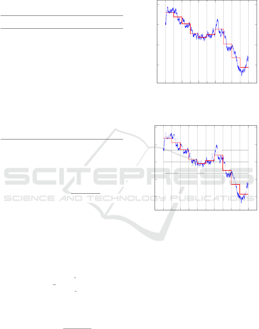
3.2 Symbolic Aggregate Approximation

The Symbolic Aggregate approXimation (SAX)

method consists of two phases. In the ﬁrst phase,

SAX reduces the length of the time series using the

Piecewise Aggregate Approximation (PAA) (Figure

1) (Keogh et al., 2001). PAA divides a times series of

length n into k segments of equal size. Then it com-

putes the average value of the points inside each seg-

ment using the formula:

PAA(x) =

∗

(x+1)∗

−1

∑

i=x∗

T S(i) (6)

In the second phase, SAX performs a numeric re-

duction. In this phase, SAX normalizes the time se-

ries using the following formula:

ZNorm(x) =

T S(x) − µ

T S

(7)

After applying 7, the time series is normalized to

zero mean and unit standard deviation. In this case the

values have a Gaussian distribution. The next step is

0 200 400

600

800 1,000

−40

−20

Time

Values

Figure 1: The PAA representation of a time series. The ini-

tial time series of length 1000 is reduced to a representation

with 10 segments.

0 200 400

600

800 1,000

−2

−1

Time

Normalised values

Figure 2: The SAX representation of a time series with 10

segments and an alphabet of 4 symbols.

to compute the breakpoints that will divide the distri-

bution in intervals with equal probability. The num-

ber of intervals is equal to the size of the input al-

phabet. The breakpoints can be precomputed using

statistical tables. The ﬁnal step is to label each seg-

ment based on the interval where the associated value

belongs. This step transforms the PAA representation

into a discrete representation (Figure 2).

3.3 Complexity Invariant Distance

Batista proposed a new invariance in (Batista et al.,

2011) based on the complexity property of the two

time series. Each of the known invariances deals with

a given aspect of the time series:

• amplitude/offset

KDIR 2016 - 8th International Conference on Knowledge Discovery and Information Retrieval

338

• local scaling (warping)

• global (uniform) scaling

• phase (rotation)

• occlusion (outlier)

• complexity

Batista assumes that the complexity could refer to

the number of peaks and valleys and shows that in

many cases complex time series are closer to simple

time series because the peaks and the valleys are not

perfectly aligned. Because of this, he proposed a fac-

tor that will increase or decrease the distance between

two time series given theirs complexity. The next step

was to compute the complexity of a time series. For

this, he approximates the complexity by stretching the

time series and computing the length of the resulting

line using the formula:

CE(T S) =

n−1

∑

i=1

(T S(i) − T S(i + 1))

(8)

The complexity factor (CF) between two time se-

ries is computed as following:

CF(A, B) =

max{CE(A),CE(B)}

min{CE(A),CE(B)}

(9)

4 PROPOSED DISTANCE

By default, LCSS distance deals with the local scaling

invariance and with the occlusion invariance. The lo-

cal scaling invariance refers to ﬁnding similar points

from the two time series that are not locally aligned in

the time axis. The radius of the Sakoe and Chiba re-

gion represents the maximum allowed misalignment.

The occlusion invariance refers to skipping points

from one time series that are not similar with the

points from the other time series. This helps in dis-

carding outliers. To deal with the amplitude and off-

set invariance the two time series needs to be normal-

ized. If they are normalized with Z-Normalization

then the mean will become zero and the standard devi-

ation will become one. In this case, the recommended

value for ε will be always one, which cannot be the

best choice for every dataset. Also ε should depend

on the domain that contains the values of the com-

pared points. If the domain is rare then ε should be

greater so as to ignore small differences. Otherwise if

the domain is dense then ε should be smaller.

To deal with this problem we propose to use a

discretization technique before computing LCSS. The

discretization is similar to the second phase from

SAX. The values from the time series are transformed

into symbols from a ﬁnite alphabet. Two symbols are

considered equal if the absolute difference between

the associated integer values is less than or equal to

one.

The second improvement that we propose is the

addition of a threshold value. When the partially com-

puted distance is over the given threshold then we can

stop the rest of the computation and save time. In a

classiﬁcation task the unlabelled time series is com-

pared to a set of labelled time series. The threshold

is dynamically set to the smallest distance found so

far between the unlabelled time series and a labelled

time series. The pseudo-code with the threshold is

presented in algorithm 5.

Algorithm 5 : The approximate length of LCSS with Sakoe

and Chiba region and threshold.

1: function lcss

(A, B, n, radius, threshold)

2: w ← 2 ∗ radius + 1

3: k ← 1

4: v[0..w + 1] ← 0

5: for i ← 1, n do

6: prev ← v

7: k ← max(1, radius − i)

8: start ← max(1, i − radius)

9: start ← min(n, i + radius)

10: for j ← start, end do

11: if |A[i] − B[ j]| ≤ 1 then

12: v[k] ← prev[k] + 1

13: else

14: v[k] ← max(prev[k + 1], v[k − 1])

15: if v[k − 1] + n − i ≤ threshold then

16: return −1

17: k ← k + 1

18: return v[k − 1]

5 RESULTS AND EVALUATION

For all the experiments that we run, we used the clas-

siﬁer k-nearest neighbours (KNN) with k=1 because

it is the most used in the ﬁeld of time series (Rakthan-

manon et al., 2012). We choose the classiﬁer imple-

mentation from Weka library (Hall et al., 2009). Also

the algorithms are implemented in Java based on the

description in their source articles. The source code

is available online at (Hasna, 2015).

In the ﬁrst experiment we tried to ﬁnd the best

value for the parameters of the proposed distances:

constrained LCSS (LCSS), constrained LCSS with

CID (CID-LCSS), discrete LCSS (dLCSS) and dis-

crete LCSS with CID (CID-dLCSS). For this experi-

ment we used the train instances from the benchmark

The Longest Common Subsequence Distance using a Complexity Factor

339

Table 2: The best value for the parameters with the corresponding classiﬁcation error percentage for LCSS, CID-LCSS,

dLCSS and CID-dLCSS.

LCSS CID-LCSS dLCSS CID-dLCSS

Datasets R ε Error R ε Error R |A| Error R |A| Error

50words 10 0,2 21,11 10 0,2 20,44 10 32 22,22 10 16 21,33

Adiac 1 0,05 38,71 1 0,05 35,12 1 256 49,23 1 256 47,69

Beef 2 0,1 46,66 2 0,1 53,33 1 32 46,67 1 32 53,33

CBF 1 0,1 3,33 1 0,2 0 6 512 0 1 8 0

ChlorineConcentration 0 0,2 27,83 0 0,2 28,9 0 32 30,41 0 16 31,91

CinCECGtorso 1 0,8 10 2 0,8 7,5 2 16 12,5 1 16 12,5

Coffee 4 0,1 0 1 0,2 0 1 32 0 1 32 0

CricketX 9 0,4 22,56 5 0,4 20,51 9 16 23,59 6 16 21,03

CricketY 9 0,4 23,33 6 0,4 27,94 9 8 29,74 5 8 29,49

CricketZ 8 0,4 23,84 5 0,4 22,56 10 8 23,59 9 8 20,51

DiatomSizeReduction 1 0,00625 6,25 1 0,00625 6,25 1 32 6,25 1 32 6,25

ECG200 4 0,4 12 2 0,2 12 4 16 12 4 16 10

ECGFiveDays 8 0,0125 8,69 0 0,00625 8,69 0 8 17,39 0 8 17,39

FaceAll 6 0,8 2,14 9 0,4 1,78 6 8 1,79 5 8 2,32

FaceFour 1 0,2 4,16 1 0,2 8,33 1 8 4,17 6 8 0

FacesUCR 10 0,4 3,5 7 0,4 4 9 8 3 9 16 2,5

ﬁsh 7 0,05 13,14 5 0,025 13,14 4 32 14,86 3 64 16

GunPoint 1 0,2 2 2 0,2 2 3 32 0 2 32 0

Haptics 1 0,4 46,45 8 0,4 43,87 5 8 48,39 2 32 47,1

InlineSkate 5 0,2 48 9 0,00625 44 8 64 50 9 64 47

ItalyPowerDemand 5 0,1 7,46 5 0,025 2,98 5 64 4,48 5 8 5,97

Lighting2 1 0,1 16,66 3 0,1 16,66 9 32 16,67 1 16 21,67

Lighting7 10 0,4 27,14 1 0,1 24,28 1 16 31,43 2 32 31,43

MALLAT 1 0,4 1,81 1 0,4 1,81 1 8 9,09 3 64 5,46

MedicalImages 8 0,2 30,97 4 0,2 29,92 5 32 29,13 9 32 26,51

MoteStrain 4 0,0125 10 2 0,8 15 3 128 10 2 32 20

OliveOil 1 0,00625 6,66 1 0,00625 6,66 1 512 10 1 512 10

OSULeaf 10 0,2 18 10 0,2 19,5 10 32 18 10 16 19

SonyAIBORobotSurface1 2 0,4 10 0 0,00625 0 2 16 10 0 16 0

SonyAIBORobotSurface2 8 0,05 7,4 2 0,05 7,4 2 8 7,41 2 8 7,41

StarLightCurves 10 0,1 10,9 1 0,025 5 5 32 12,2 1 512 5,1

SwedishLeaf 4 0,2 10,8 3 0,2 10,6 10 16 15,2 10 16 13,4

Symbols 6 0,2 4 10 0,025 0 10 16 0 1 64 0

SyntheticControl 7 0,8 2,66 4 0,8 3 4 8 5,67 5 32 3

Trace 3 0,2 2 0 0,4 0 4 32 1 4 32 1

TwoLeadECG 7 0,2 4,34 7 0,1 4,34 3 32 4,35 7 32 4,35

TwoPatterns 9 0,8 0 10 0,2 0 7 16 0 8 8 0

uWaveGestureLibraryX 6 0,4 23,99 7 0,2 21,54 10 16 25 7 16 22,77

uWaveGestureLibraryY 4 0,4 28,01 8 0,4 25,44 7 32 27,68 6 32 26,23

uWaveGestureLibraryZ 8 0,4 26,56 8 0,4 24,44 8 16 28,35 9 32 27,01

wafer 1 0,2 0,1 2 0,2 0 1 4 0 1 4 0

WordsSynonyms 9 0,4 22,47 8 0,2 23,97 9 32 24,35 9 8 24,35

yoga 8 0,05 12 10 0,05 11,66 8 128 13 10 128 14

AVERAGE 15,06 14,29 16,25 15,69

datasets (Chen et al., 2015) and we apply the hold-

one-out validation i.e. one instance is used for testing

and the rest of the instances are used for training the

classiﬁer.

The best values for the parameters are searched in

the intervals presented in Table 1. The chosen values

for the parameters and the corresponding classiﬁca-

tion error percentage are shown in the Table 2.

Table 1: The tested values for the distances parameters.

Parameters Tested values

radius (R) 1%, 2%, 3%, 4%, 5%, 6%, 7%, 8%, 9%, 10%

alphabet size (|A|) 4, 8, 16, 32, 64, 128, 256, 512

epsilon (ε) 0.00625, 0.0125, 0.025, 0.05, 0.1, 0.2, 0.4, 0.8

Table 2 that for 36 from 43 datasets it is better

to apply the complexity invariant factor (CID) and

among them there are 15 cases where the results are

KDIR 2016 - 8th International Conference on Knowledge Discovery and Information Retrieval

340

Table 3: The classiﬁcation error percentage on the test instances for the 43 benchmark datasets.

Datasets DTW-full LCSS-full LCSS CID-LCSS dLCSS CID-dLCSS

50words 31,94 20,76 20,44 19,78 22,19 20,44

Adiac 39,66 75,84 38,61 35,55 48,84 46,03

Beef 50,3 45,7 26,66 26,66 23,33 23,33

CBF 0,67 1,67 12 1,77 1,44 2,77

ChlorineConcentration 35,45 30,13 28,17 29,16 31,97 30,75

CinCECGtorso 32,64 7,15 6,66 5,14 12,17 9,92

Coffee 1,11 2,11 7,14 0 10,71 10,71

CricketX 23,54 24,46 26,15 26,41 28,2 24,35

CricketY 26,2 24,3 22,05 24,35 26,92 25,38

CricketZ 22,82 23,39 24,35 24,87 28,97 23,33

DiatomSizeReduction 4,19 6,55 8,82 8,49 5,55 5,22

ECG200 20,13 14,15 9 10 11 13

ECGFiveDays 23,97 13,45 28,57 25,43 10,56 17,88

FaceAll 5,68 2,02 21,06 19,11 22,18 22,48

FaceFour 15,1 5,27 6,81 7,95 6,81 6,81

FacesUCR 10,15 4,44 4,63 5,56 4,82 6,73

ﬁsh 23,68 13,73 10,28 8 13,71 12,57

GunPoint 12,4 6,53 4 2,66 2 2

Haptics 60,99 59,44 65,9 62,66 63,63 61,68

InlineSkate 60,49 57,55 56,72 54,54 60,72 59,09

ItalyPowerDemand 7,74 6,26 13,31 15,74 10,78 7,67

Lighting2 17,7 24,51 14,75 16,39 18,03 18,03

Lighting7 30,16 34,22 32,87 35,61 31,5 34,24

MALLAT 5,78 7,07 10,06 9,42 13,81 8,31

MedicalImages 25,88 31,3 32,36 31,97 31,97 29,47

MoteStrain 16,79 12,18 18,53 14,29 17,33 18,69

OliveOil 13,93 60 16,66 16,66 13,33 13,33

OSULeaf 38,27 22,14 23,55 24,38 24,79 24,79

SonyAIBORobotSurface1 19,91 24,81 28,95 9,48 27,12 10,15

SonyAIBORobotSurface2 15,39 16,92 22,24 10,59 15,74 14,69

StarLightCurves 8,57 14,07 11,26 5,82 14,31 6,14

SwedishLeaf 21,36 11,11 11,04 11,2 14,88 12,64

Symbols 5,92 6,58 6,53 4,42 5,32 7,23

SyntheticControl 0,89 3,06 5,33 4,33 5,33 7,33

Trace 0,03 1,91 3 6 1 1

TwoLeadECG 8,17 11,73 10,88 8,78 18,96 8,95

TwoPatterns 0 0,14 0,07 0,2 0,07 0,1

uWaveGestureLibraryX 27,24 22,48 23,42 21,97 23,64 22,22

uWaveGestureLibraryY 37,68 31,07 31,29 28,42 31,63 29,34

uWaveGestureLibraryZ 34,35 30,61 30,43 28,53 31,74 29,87

wafer 1,6 0,39 0,92 0,82 0,35 0,4

WordsSynonyms 35,12 24,87 24,6 25,7 28,21 26,64

yoga 15,12 13,43 14 13,8 13,96 14,2

AVERAGE 20,66 19,75 18,93 17,27 19,29 17,9

signiﬁcantly better (over 5% improvement). In 9

cases it is better to not use CID and this happens be-

cause the instances from the same class have different

levels of noise which implies different levels of com-

The Longest Common Subsequence Distance using a Complexity Factor

341

plexity.

In the second experiment we want to ﬁnd out if the

assumptions made on the train instances are still valid

for the test instances. Also we want to compare the re-

sults for LCSS, CID-LCSS, dLCSS and CID-dLCSS

with the published results in (Bagnall et al., 2016) for

LCSS-full (no constraint region) and for the state of

the art DTW-full (no constrain region) and COTE. For

this experiment we used for the parameters of LCSS,

CID-LCSS, dLCSS and CID-dLCSS the values ob-

tain in the previous experiment. The classiﬁer learns

from the train set and it is tested on the test set. The

split between test and train is already made on the

benchmark datasets. In Table 3 there are presented the

classiﬁcation error percentages for the baseline meth-

ods: DTW-full and LCSS-full and for our methods:

LCSS, CID-LCSS, dLCSS and CID-dLCSS.

As we can see from the results, in 32 cases (75%)

the magnitude order between the errors of LCSS and

CID-LCSS on the test set remains the same as on the

train sets. In the case of dLCSS and CID-dLCSS there

are 29 datasets (67%) where the magnitude order is

preserved. When we compare CID-LCSS with the

baseline LCSS method (LCSS-full) there are 19 cases

(37%) where CID-LCSS is better than LCSS-full.

Among this cases there are 17 where the difference

is signiﬁcant (more than 5% improvement). When we

compare CID-dLCSS with the baseline LCSS method

(LCSS-full) there are 32 cases (75%) where CID-

dLCSS is better than LCSS-full. Among this cases

there are the same 17 where the difference is signiﬁ-

cant (more than 5% improvement).

In the third experiment (Table 4) we compare

the improvement made by the proposed threshold for

the distances: LCSS, CID-LCSS, dLCSS and CID-

dLCSS. We use the same classiﬁer, train and test in-

stances and distances parameters as in the previous

experiment. We ran this experiment two times and

count the number of comparisons between the points

(line 11 from Algorithm 5). In the ﬁrst run, the dis-

tances use the threshold (lines 15 and 15 from Algo-

Table 4: The number of benchmark datasets for which the

percentage of skipped comparisons is in the given interval.

Intervals LCSS CID-LCSS dLCSS CID-dLCSS

0-10 1 0 0 0

10-20 4 4 1 1

20-30 1 4 1 0

30-40 4 0 4 4

40-50 5 5 5 5

50-60 7 14 15 11

60-70 12 3 10 12

70-80 6 8 5 8

80-90 2 4 1 1

90-100 1 1 1 1

rithm 5) and in the second run the distances didn’t use

the threshold.

From the results presented in Table 4 we can see

that in the majority of the cases (> 50%), we skipped

between 50% and 70% of the comparisons. In more

than 65% of the cases we skipped at least 50% of the

comparisons. The number of comparisons is corre-

lated with the computation time and this means that

we doubled the computation speed in more than 65%

of the cases.

The computation time depends on internal factors

(ex: the similarity between the two time series, the

length of the time series etc.) and external factors

(ex: the language in which the algorithms are writ-

ten, the hardware of the machine where the experi-

ments are run etc.). Taking this into consideration,

for the ﬁrst run, the smallest computation time is 0.04

ms (ItalyPowerDemand) and the longest computation

time is 315.42 ms (StarLightCurves). For the second

run, when we don’t use the threshold, the compu-

tation time is between 0.07 ms (ItalyPowerDemand)

and 1028.67 ms (StarLightCurves).

6 CONCLUSIONS

In this paper we have made a comparison between

different LCSS based distances and we have demon-

strated that applying a complexity factor to the LCSS

distance can improve the accuracy of the classiﬁca-

tion. Also we showed that using a region constraint

and a threshold value for the distance not only im-

prove the speed of classiﬁcation, but also reduce the

classiﬁcation error rate.

All the distances used in the experiments

stretches/compress one time series so as to get the best

alignment with the second time series. The main dif-

ference between DTW and LCSS is the expressive-

ness of the distance value. In the case of DTW dis-

tance, we perform a sum of the distances between the

best aligned points from the two time series, but for

computing LCSS we perform a count of the similar

points. This implies that DTW distance is more sen-

sible to the differences between the two time series.

Whereas LCSS distance can skip more easily the out-

liers from the time series. This two properties are in

opposition and choosing the best distance depends on

the type of the datasets.

Like in other classiﬁcation problems, the results

cannot be the best for each of the datasets. In the

above experiments we choose the distance that per-

forms the best in the training step. In the future we

want to search for the meta-features of the datasets

that will help us decide in which situation it is bet-

KDIR 2016 - 8th International Conference on Knowledge Discovery and Information Retrieval

342

ter to use the proposed distances without running the

initial training step.

REFERENCES

Bagnall, A., Bostrom, A., Large, J., and Lines, J. (2016).

The Great Time Series Classiﬁcation Bake Off: An

Experimental Evaluation of Recently Proposed Algo-

rithms. Extended Version.

Batista, G. E., Wang, X., and Keogh, E. J. (2011). A

Complexity-Invariant Distance Measure for Time Se-

ries. In SDM, volume 11, pages 699–710. SIAM.

Chen, Y., Keogh, E., Hu, B., Begum, N., Bag-

nall, A., Mueen, A., and Batista, G. (2015).

The UCR time series classiﬁcation archive.

www.cs.ucr.edu/∼eamonn/time series data/.

Hall, M., Frank, E., Holmes, G., Pfahringer, B., Reutemann,

P., and Witten, I. H. (2009). The weka data min-

ing software: An update. SIGKDD Explor. Newsl.,

11(1):10–18.

Hasna, O. L. (2015). The time series math library.

github.com/octavian-h/time-series-math/.

Hirschberg, D. S. (1975). A linear space algorithm for com-

puting maximal common subsequences. 18(6):341–

343.

Itakura, F. (1975). Minimum prediction residual principle

applied to speech recognition. 23(1):67–72.

Keogh, E., Chakrabarti, K., Pazzani, M., and Mehrotra, S.

(2001). Dimensionality reduction for fast similarity

search in large time series databases. 3(3):263–286.

Lin, J., Keogh, E., Lonardi, S., and Chiu, B. (2003). A sym-

bolic representation of time series, with implications

for streaming algorithms. In Proceedings of the 8th

ACM SIGMOD Workshop on Research Issues in Data

Mining and Knowledge Discovery, pages 2–11. ACM.

Rakthanmanon, T., Campana, B., Mueen, A., Batista, G.,

Westover, B., Zhu, Q., Zakaria, J., and Keogh, E.

(2012). Searching and mining trillions of time se-

ries subsequences under dynamic time warping. In

Proceedings of the 18th ACM SIGKDD International

Conference on Knowledge Discovery and Data Min-

ing, pages 262–270. ACM.

Sakoe, H. and Chiba, S. (1978). Dynamic programming

algorithm optimization for spoken word recognition.

26(1):43–49.

Vlachos, M., Kollios, G., and Gunopulos, D. (2002). Dis-

covering similar multidimensional trajectories. In

Data Engineering, 2002. Proceedings. 18th Interna-

tional Conference on, pages 673–684. IEEE.

The Longest Common Subsequence Distance using a Complexity Factor

343