
Discovering Data Lineage from Data Warehouse Procedures
Kalle Tomingas, Priit Järv and Tanel Tammet
Tallinn University of Technology, Ehitajate tee 5, Tallinn 19086, Estonia
Keywords: Data Warehouse, Data Lineage, Dependency Analysis, Data Flow Visualization.
Abstract: We present a method to calculate component dependencies and data lineage from the database structure and
a large set of associated procedures and queries, independently of actual data in the data warehouse. The
method relies on the probabilistic estimation of the impact of data in queries. We present a rule system
supporting the efficient calculation of the transitive closure. The dependencies are categorized, aggregated
and visualized to address various planning and decision support problems. System performance is evaluated
and analysed over several real-life datasets.
1 INTRODUCTION
System developers and managers are facing similar
data lineage and impact analysis problems in complex
data integration, business intelligence and data
warehouse environments where the chains of data
transformations are long and the complexity of
structural changes is high. The management of data
integration processes becomes unpredictable and the
costs of changes can be very high due to the lack of
information about data flows and the internal
relations of system components. Important contextual
relations are encoded into data transformation queries
and programs (SQL queries, data loading scripts,
etc.). Data lineage dependencies are spread between
different systems and frequently exist only in
program code or SQL queries. This leads to
unmanageable complexity, lack of knowledge and a
large amount of technical work with uncomfortable
consequences like unpredictable results, wrong
estimations, rigid administrative and development
processes, high cost, lack of flexibility and lack of
trust.
We point out some of the most important and
common questions for large DW which usually
become a topic of research for system analysts and
administrators:
Where does the data come or go to in/from a
specific column, table, view or report?
When was the data loaded, updated or calculated
in a specific column, table, view or report?
Which components (reports, queries, loadings and
structures) are impacted when other components
are changed?
Which data, structure or report is used by whom
and when?
What is the cost of making changes?
What will break when we change something?
The ability to find ad-hoc answers to many day to
day questions determines not only the management
capabilities and the cost of the system, but also the
price and flexibility of making changes.
The goal of our research is to develop reliable and
efficient methods for automatic discovery of
component dependencies and data lineage from the
database schemas, queries and data transformation
components by automated analysis of actual program
code. This requires probabilistic estimation of the
measure of dependencies and the aggregation and
visualization of the estimations.
2 RELATED WORK
Impact analysis, traceability and data lineage issues
are not new. A good overview of the research
activities of the last decade is presented in an article
by (Priebe, 2011). We can find various research
approaches and published papers from the early
1990’s with methodologies for software traceability
(Ramesh, 2001). The problem of data lineage tracing
in data warehousing environments has been formally
founded by Cui and Widom (Cui, 2000; Cui 2003).
Overview of data lineage and data provenance tracing
studies can be found in book by Cheney et al.
(Cheney, 2009). Data lineage or provenance detail
Tomingas, K., Järv, P. and Tammet, T.
Discovering Data Lineage from Data Warehouse Procedures.
DOI: 10.5220/0006054301010110
In Proceedings of the 8th International Joint Conference on Knowledge Discovery, Knowledge Engineering and Knowledge Management (IC3K 2016) - Volume 1: KDIR, pages 101-110
ISBN: 978-989-758-203-5
Copyright
c
2016 by SCITEPRESS – Science and Technology Publications, Lda. All rights reserved
101
levels (e.g. coarse-grained vs fine-grained), question
types (e.g why-provenance, how-provenance and
where-provenance) and two different calculation
approaches (e.g. eager approach vs lazy approach)
discussed in multiple papers (Tan, 2007; Benjelloun,
2006) and formal definitions of why-provenance
given by Buneman et al. (Buneman, 2001). Other
theoretical works for data lineage tracing can be
found in (Fan, 2003; Giorgini, 2008). Fan and
Poulovassilis developed algorithms for deriving
affected data items along the transformation pathway
[6]. These approaches formalize a way to trace tuples
(resp. attribute values) through rather complex
transformations, given that the transformations are
known on a schema level. This assumption does not
often hold in practice. Transformations may be
documented in source-to-target matrices
(specification lineage) and implemented in ETL tools
(implementation lineage). Woodruff and Stonebraker
create solid base for the data-level and the operators
processing based the fine-grained lineage in contrast
to the metadata based lineage calculation in their
research paper (Woodruff, 1997).
Other practical works that are based on conceptual
models, ontologies and graphs for data quality and
data lineage tracking can be found in (Skoutas, 2007;
Tomingas, 2014; Vassiliadis, 2002; Widom, 2004).
De Santana proposes the integrated metadata and the
CWM metamodel based data lineage documentation
approach (de Santana, 2004). Tomingas et al. employ
the Abstract Mapping representation of data
transformations and rule-based impact analysis
(Tomingas, 2014).
Priebe et al. concentrates on proper handling of
specification lineage, a huge problem in large-scale
DWH projects, especially in case different sources
have to be consistently mapped to the same target
(Priebe, 2011). They propose a business information
model (or conceptual business glossary) as the
solution and a central mapping point to overcome
those issues.
Scientific workflow provenance tracking is
closely related to data lineage in databases. The
distinction is made between coarse-grained, or
schema-level, provenance tracking (Heinis, 2008)
and fine-grained or data instance level tracking
(Missier, 2008). The methods of extracting the
lineage are divided to physical (annotation of data by
Missier et al.) and logical, where the lineage is
derived from the graph of data transformations
(Ikeda, 2013).
In the context of our work, efficiently querying of
the lineage information after the provenance graph
1
http://www.goldparser.org/
has been captured, is of specific interest. Heinis and
Alonso present an encoding method that allows
space-efficient storage of transitive closure graphs
and enables fast lineage queries over that data
(Heinis, 2008). Anand et al. propose a high level
language QLP, together with the evaluation
techniques that allow storing provenance graphs in a
relational database (Anand, 2010).
3 WEIGHT ESTIMATION
The inference method of the data flow and the impact
dependencies that presented in this paper is part of a
larger framework of a full impact analysis solution.
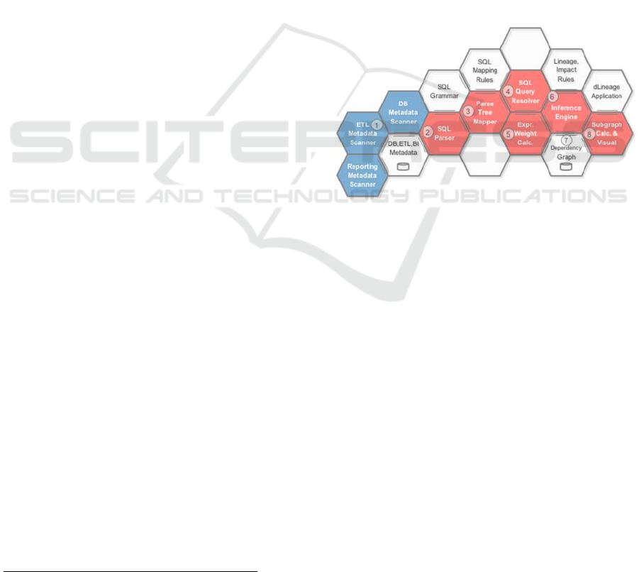
The core functions of the system architecture are built
upon the following components presented in the
Figure 1 and described in detail in our previous works
(Tomingas, 2014; Tomingas, 2015).
Figure 1: Impact analysis system architecture components.
The core functions of the system architecture are
built upon the following components in the Figure 1:
1. Scanners collect metadata from different systems
that are part of DW data flows (DI/ETL processes,
data structures, queries, reports etc.).
2. The SQL parser is based on customized
grammars, GoldParser
1
parsing engine and the Java-
based XDTL engine.
3. The rule-based parse tree mapper extracts and
collects meaningful expressions from the parsed text,
using declared combinations of grammar rules and
parsed text tokens.
4. The query resolver applies additional rules to
expand and resolve all the variables, aliases, sub-
query expressions and other SQL syntax structures
which encode crucial information for data flow
construction.
5. The expression weight calculator applies rules to
calculate the meaning of data transformation, join and
KDIR 2016 - 8th International Conference on Knowledge Discovery and Information Retrieval
102

filter expressions for impact analysis and data flow
construction.
6. The probabilistic rule-based reasoning engine
propagates and aggregates weighted dependencies.
7. The open-schema relational database using
PostgreSQL for storing and sharing scanned,
calculated and derived metadata.
8. The directed and weighted sub-graph
calculations, and visualization web based UI for data
lineage and impact analysis applications.
In the stages preceding the impact estimation,
inference and aggregation the data structure
transformations are parsed and extracted from queries
and stored as formalized, declarative mappings in the
system.
To add additional quantitative measures to each
column transformation or column usage in the join
and filter conditions we evaluate each expression and
calculate the transformation and filter weights for
those.
Definition 1. The column transformation weight
Wt is based on the similarity of each source column
and column transformation expression: the calculated
weight expresses the source column transfer rate or
strength. The weight is calculated on scale [0,1]
where 0 means that the data is not transformed from
source (e.g. constant assignment in a query) and 1
means that the source is copied to the target directly,
ie. no additional column transformations are detected.
Definition 2. The column filter weight Wf is based
on the similarity of each filter column in the filter
expression where the calculated weight expresses the
column filtering strength. The weight is calculated on
the scale [0,1] where 0 means that the column is not
used in the filter and 1 means that the column is
directly used in the filter predicate, ie. no additional
expressions are involved.
The general column weight W algorithm in each
expression for Wt and Wf components is calculated
as a column count ratio over all the expression
component counts (e.g. column count, constant count,
function count, predicate count).
The counts are normalized using the FncList
evaluation over a positive function list (e.g. CAST,
ROUND, COALESCE, TRIM etc.). If the FncList
member is in a positive function list, then the
normalization function reduces the according
component count by 1 to pay a smaller price in case
the function used does not have a significant impact
to column data.
Definition 3. A primitive data transformation
operation is a data transformation between a source
column X and a target column Y in a transformation
set M (mapping or query) having the expression
similarity weight Wt.
Definition 4. The column X is a filter condition in
a transformation set M with the filter weight Wf if the
column is part of a JOIN clause or WHERE clause in
the queries corresponding to M.
4 RULE SYSTEM AND
DEPENDENCY CALCULATION
The primitive transformations captured from the
source databases form a graph G
O
with nodes N
representing database objects and edges E
O
representing primitive transformations (see
Definition 3). We define relations :
→ and
:
→ connecting edges to source nodes and
target nodes, respectively. We define label relations
:
→
|
and
:
→ 0,1. Formally, this graph is an edge-
labeled directed multigraph.
In the remainder of the article, we will use the
following intuitive notation: e.X and e.Y to denote
source and target objects of a transformation
(formally, and ). e.M is the set of source
transformations (). e.W is the weight assigned to
the edge ().
The knowledge inferred from the primitive
transformations forms a graph
,
where
E
L
is the set of edges e that represent data flow
(lineage). We define relations X, Y, M and W the same
way as with the graph G
O
and use the e.R notation
where R is one of the relations {X, Y, M, W}.
Additionally, we designate the graph
,
∪
to represent the impact relations
between database components. It is a superset of G
L
where E
L
is the set of additional edges inferred from
column usage in filter expressions.
4.1 The Propagation Rule System
First, we define the rule to map the primitive data
transformations to our knowledge base. This rule
includes aggregation of multiple edges between pairs
of nodes.
Let
,
∈
|.,. be
the set of edges connecting nodes x, y in the graph G
O
.
∀, ∈
,
∅ ⟹∃′∈
(R1),
such that
′. ⋀′. (R1.1)
Discovering Data Lineage from Data Warehouse Procedures
103

′. ∪
∈
,
. (R1.2)
′. . | ∈
,
(R1.3)
An inference using this rule should be understood
as ensuring that our knowledge base satisfies the rule.
From an algorithmic perspective, we create edges e’
into the set E
L
until R1 is satisfied.
Definition 5. The predicate Parent(x, p) is true if
node p is the parent of node x in the database schema.
Filter conditions are mapped to edges in the
impact graph G
I
.
Let
,
|
,
⋀
be the set of nodes that are
filter conditions for the mapping M with parent p. Let
,
|
,
∧ } be
the set of nodes that represent the target columns of
mapping M. To assign filter weights to columns, we
define the function
: → 0, 1.
∀, ′ ∈
,
∅⋀
,
∅⟹∃′∈
(R2
)
such that
′. ⋀′. ′ (R2.1)
′. (R2.2)
′.
|∈
,
|∈
,
(R2.3)
The primitive transformations mostly represent
column-level (or equivalent) objects that are adjacent
in the graph (meaning, they appear in the same
transformation or query and we have captured the
data flow from one to another). The same applies to
impact information inferred from filter conditions.
From this knowledge, the goal is to additionally:
● propagate information through the database
structure upwards, to view data flows on a more
abstract level (such as, table or schema level)
● calculate the dependency closure to answer
lineage queries
Unless otherwise stated, we treat the graphs G
L
and G
I
similarly from this point. It is implied that the
described computations are performed on both of
them. The set E refers to the edges of either of those
graphs.
Let
,
∈
|
. ,
⋀
.,’ be the set of edges where the
source nodes share a common parent p and the target
nodes share a common parent p’.
∀, ′ ∈
,
∅⟹∃′ ∈ (R3),
such that
′. ⋀′. ′ (R3.1)
. ∪
∈
,
. (R3.2)
′.
∑
∈
,
.
|
,
|
(R3.3)
4.2 The Dependency Closure
Online queries from the dataset require finding the
data lineage of a database item without long
computation times. For displaying both the lineage
and impact information, we require that all paths
through the directed graph that include a selected
component are found. These paths form a connected
subgraph. Further manipulation (see Section 4.3) and
data display is then performed on this subgraph.
There are two principal techniques for retrieving
paths through a node (Heinis, 2008):
● connect the edges recursively, forming the paths
at query time. This has no additional storage
requirements, but is computationally expensive
● store the paths in materialized form. The paths can
then be retrieved without recursion, which speeds
up the queries, but the materialized transitive
closure may be expensive to store.
Several compromise solutions that seek to both
efficiently store and query the data have been
published (Heinis, 2008; Anand, 2010). In general,
the transitive closure is stored in a space efficient
encoding that can be expanded quickly at the query
time.
We have incorporated elements from the pointer
based technique introduced in (Anand, 2010). The
paths are stored in three relations:
Node(N1,P_dep,P_depc),
Dep(P_dep,N2)and DepC(P_depc,P_dep).
Immediate dependen-cies of a node are stored in the
Dep relation, with the pointer P_dep in the Node
relation referring to the dependency set. The full
transitive dependency closure is stored in the DepC
relation by storing the union of the pointers to all of
the immediate dependency sets of nodes along the
paths leading to a selected node.
We can define the dependency closure recursively
as follows. Let D*
k
be the dependency closure of node
k. Let D
k
be the set of immediate dependencies such
that
| ∈ , . , . .
If
∅ then
∗
∅ .
Else if
∅ then
∗
∪∪
∈
∗
.
The successors S
j
(including non-immediate) of a
node j are found as follows:
|∈
∗
The materialized storage of the dependency
closure allows building the successor set cheaply, so
it does not need to be stored in advance. Together
with the dependency closure they form the connected
maximal subgraph that includes the selected node.
KDIR 2016 - 8th International Conference on Knowledge Discovery and Information Retrieval
104

We put the emphasis on the fast computation of
the dependency closure with the requirement that the
lineage graph is sparse (|| ∼ ||). We have omitted
the more time-consuming redundant subset and
subsequence detection techniques of Anand et al.
(Anand, 2009). The subset reduction has ||
time complexity which is prohibitively expensive if
the number of initial unique dependency sets || is
on the order of 10
5
as is the case in our real world
dataset.
The dependency closure is computed by:
1. Creating a partial order L of the nodes in the
directed graph G
I
. If the graph is cyclic then we
need to transform it to a DAG by deleting an edge
from each cycle. This approach is viable, if the
graph contains relatively few cycles. The
information lost by deleting the edges can be
restored at a later stage, but this process is more
expensive than computing the closure on a DAG.
2. Creating the immediate dependency sets for each
node using the duplicate-set reduction algorithm
(Anand, 2009).
3. Building the dependency closures for each node
using the partial order L, ensuring that the
dependency sets are available when they are
needed for inclusion in the dependency closures
of successor nodes (Algorithm 1).
4. If needed, restoring deleted cyclic edges and
incrementally adding dependencies that are
carried by those edges using breadth-first search
in the direction of the edges.
Algorithm 1. Building the pointer-encoded
dependency closure:
Input: L - partial order on G
I
;
{D
k
|k∈N} - immediate dependency sets
Output: D*
k
- dependency closures
for each node k∈N
for node k in L:
D*
k
= {D
k
}
for j in D
k
:
D*
k
= D*
k
∪D*
j
This algorithm has linear time complexity
|| || if we disregard the duplicate set
reduction. To reduce the required storage, if
∗
∗
for any then we may replace one of them
with a pointer to the other. The set comparison
increases the worst case time complexity to ||
.
To extract the nodes along the paths that go
through a selected node N, one would use the
following queries:
select Dep.N2 --predecessor nodes
from Node, DepC, Dep
where Dep.P_dep = DepC.P_dep
and DepC.P_depc = Node.P_depc
and Node.N1 = N
select Node.N1 --successor nodes
from Node, DepC, Dep
where Node.P_depc = DepC.P_depc
and DepC.P_dep = Dep.P_dep
and Dep.N2 = N
4.3 Visualization of the Lineage and
Impact Graphs
The visualization of the connected subgraph
corresponding to a node j is created by fetching the
path nodes
∗
∪
and the edges along those
paths
∈|.∈
⋀. ∈
from the
appropriate dependency graph (impact or lineage).
The graphical representation allows filtering a subset
of nodes in the application, by node type, although the
filtering technique discussed here is generic and
permits arbitrary criteria. Any nodes not included in
graphical display are replaced by transitive edges
bypassing these nodes to maintain the connectivity of
the dependencies in the displayed graph.
Let
,
be the connected sub graph for
the selected node j. We find the partial transitive
graph G
j
’ that excludes the filtered nodes P
filt
as
follows (Algorithm 2):
Algorithm 2. Building the filtered subgraph with
transitive edges.
Input: G
j
, P
filt
Output: G
j
’ = (P
j
’, E
j
’)
E
j
’ = E
j
P
j
’ = ∅
for node n in P
j
:
if n ∈ P
filt
:
for e in {e ∈ E
j
’| e.Y = n}:
for e’ in {e’ ∈ E
j
’| e’.X = n}:
create new edge e’’ ( e’’.X = e.X,
e’’.Y = e’.Y, e’’.W = e.W * e’’.W)
E
j
’ = E
j
’ ⋃ {e’’}
E
j
’= E
j
’ \ {e}
for e’ in {e’ ∈ E
j
’| e’.X = n}:
E
j
’ = E
j
’ \ {e’}
else:
P
j
’ = P
j
’ ⋃ {n}
This algorithm has the time complexity of O(|Pj|
+ |Ej|) and can be performed on demand when the user
changes the filter settings. This extends to large
dependency graphs with the assumption that |GJ| <<
|G|.
Discovering Data Lineage from Data Warehouse Procedures
105

4.4 The Semantic Layer Calculation
The semantic layer is a set of visualizations and
associated filters to localize the connected subgraph
of the expected data flows for the current selected
node. All the connected nodes and edges in the
semantic layer share the overlapping filter predicate
conditions or data production conditions that are
extracted during the edge construction to indicate not
only possible data flows (based on connections in
initial query graph), but only expected and
probabilistic data flows. The main idea of the
semantic layer is to narrow down all the possible and
expected data flows over all the connected graph
nodes by cutting down unlikely or disallowed
connections in graph, which is based on the additional
query filters and the semantic interpretation of filters
and calculated transformation expression weights.
The semantic layer of the data lineage graph will hide
irrelevant and/or highlight the relevant graph nodes
and edges, depending on the user choice and
interaction.
This has a significant impact when the underlying
data structures are abstract enough and the
independent data flows store and use independent
horizontal slices of data. The essence of the semantic
layer is to use the available query and schema
information to estimate the row level data flows
without any additional row level lineage information
which would be unavailable on schema level and
expensive or impossible to collect on the row level.
The visualization of the semantically connected
subgraph corresponding to node j is created by
fetching the path nodes
∗
∪
and the edges
along those paths
∈|.∈
⋀. ∈
from the appropriate dependency graph (impact or
lineage). Any nodes not included in the semantic
layer are removed or visually muted (by changing the
color or opacity) and the semantically connected
subgraph is returned or visualized by the user
interface.
Let
,
be the connected subgraph for
the selected node j where
,
is the
predecessor subgraph and
,
is the
successor subgraph according to the selected node j.
We calculate the data flow graph G
j
’ that is the union
of the semantically connected predecessors
′
,
and successor subgraphs
′
,
.
The semantic layer calculation is based on the
selected node filter set F
j
and calculated separately for
back (predecessor) and forward (successors)
directions by the recursive algorithm (Algorithm 3):
Algorithm 3. Building the semantic layer subgraph
using predecessor and successor functions
recursively.
Function: Predecessors
Input: n
j
, F
j
, GD
j
, GD’
j
W
min
Output: GD
j
’ = (D
j
’, ED
j
’)
F
n
= ∅
if D
j
’ = ∅ then:
D
j
’ = D
j
’ ⋃ n
j
for edge e in {e ∈ ED
j
| e.Y = n
j
F
n
= ∅
if F
j
!= ∅:
for filter f in e.{F}:
for filter f
j
in F
j
:
if f.Key = f
j
.Key & f.Val ∩
f
j
.Val:
new filter f
n
(f
n
.Key=f.Key,
f
n
.Val=f.Val, f
n
.Wgt=f.Wgt*f
j
.Wgt)
F
n
= F
n
⋃ f
n
else:
F
n
= F
n
⋃ e.{F}
if F
n
!= ∅ & e.W >= W
min
:
D
j
’ = D
j
’ ⋃ e.X
ED
j
’ = ED
j
’ ⋃ e
GD
j
’=Predecessors
(e.X,F
n
,GD
j
,GD’
j
,W
min
)
return GD
j
’
Function: Successors
Input: n
j
, F
j
, GS
j
, GS’, W
min
Output: GS
j
’ = (S
j
’, ES
j
’)
F
n
= ∅
if S
j
’ = ∅:
S
j
’ = S
j
’ ⋃ n
j
for edge e in {e ∈ ES
j
| e.X = n
j
}:
F
n
= ∅
if F
j
!= ∅ then:
for filter f in e.{F}:
for filter f
j
in F
j
:
if f.Key = f
j
.Key & f.Val ∩
f
j
.Val:
new filter f
n
(f
n
.Key=f.Key,
f
n
.Val=f.Val, f
n
.Wgt=f.Wgt*f
j
.Wgt)
F
n
= F
n
⋃ f
n
else:
F
n
= F
n
⋃ e.{F}
if F
n
!= ∅ & e.W >= W
min
:
S
j
’ = S
j
’ ⋃ e.Y
ES
j
’ = ES
j
’ ⋃ e
GS
j
’=Predecessors(e.Y,F
n
,GS
j
,GS
j
’,W
min
)
return GS
j
’
The final semantic layer subgraph is an union of
the recursively constructed predecessor
′ and
successor
′ graphs: G
j
’ = GD
j
’ ⋃ GS
j
’
KDIR 2016 - 8th International Conference on Knowledge Discovery and Information Retrieval
106
4.5 Dependency Score Calculation
We use the derived dependency graph to solve
different business tasks by calculating the selected
component(s) lineage or impact over available layers
and chosen details. Business questions like: “What
reports are using my data?”, “Which components
should be changed or tested?” or “What is the time
and cost of change?” are converted to directed
subgraph navigation and calculation tasks. The
following definitions add new quantitative measures
to each component or node in the calculation. We use
those measures in the user interface to sort and select
the right components for specific tasks.
Definition 6. Local Lineage Dependency %
(LLD) is calculated as the ratio over the sum of the
local source and target lineage weights W
t
.
∑
source
∑
source
∑
target
Local Lineage Dependency 0 % means that there
are no data sources detected for the object. Local
Lineage Dependency 100 % means that there are no
data consumers (targets) detected for the object.
Local Lineage Dependency about 50 % means that
there are equal numbers of weighted sources and
consumers (targets) detected for the object.
Definition 7. Local Impact Dependency % (LID)
is calculated as the ratio over the sum of local source
and target impact weights W(W
t,
,W
f
).
∑
source
∑
source
∑
target
5 CASE STUDIES
The previously described algorithms have been used
to implement an integrated toolset. Both the scanners
and the visualization tools have been enhanced and
tested in real-life projects and environments to
support several popular data warehouse platforms
(e.g. Oracle, Greenplum, Teradata, Vertica,
PostgreSQL, MsSQL, Sybase), ETL tools (e.g.
Informatica, Pentaho, Oracle Data Integrator, SSIS,
SQL scripts and different data loading utilities) and
business intelligence tools (e.g. SAP Business
Objects, Microstrategy, SSRS). The dynamic
visualization and graph navigation tools are
implemented in Javascript using the d3.js graphics
libraries.
Current implementation has rule system which is
implemented in PostgreSQL database using SQL
2
http://www.dlineage.com/
queries for graph calculation (rules 1-3 in section 4.1)
and specialized tables for graph storage. The DB and
UI interaction tested with the specialized pre-
calculated model (see section 4.2) but also with the
recursive queries without special storage and pre
calculations. The algorithms for interactive transitive
calculations (see sections 4.3) and semantic layer
calculation (see section 4.4) are implemented in
Javascript and works in browser for small and local
subgraph optimization or visualization. Due to space
limitations we do not stop here for discussion and the
details of case studies. Technical details and more
information can be found on our dLineage
2
online
demo site. We present different datasets processing
and performance analysis in the next section and
illustrate the application and algorithms with the
graph visualizations technique (section 5.2).
5.1 Performance Evaluation
We have tested our solution in several real-life case
studies involving a thorough analysis of large
international companies in the financial, utilities,
governance, telecom and healthcare sectors. The case
studies analyzed thousands of database tables and
views, tens of thousands of data loading scripts and
BI reports. Those figures are far over the capacity
limits of human analysts not assisted by the special
tools and technologies.
The following six different datasets with varying
sizes have been used for our system performance
evaluation. The datasets DS1 to DS6 represent data
warehouse and business intelligence data from
different industry sectors and is aligned according to
the dataset size (Table 1). The structure and integrity
of the datasets is diverse and complex, hence we have
analyzed the results at a more abstract level (e.g. the
number of objects and processing time) to evaluate
the system performance under different conditions.
Table 1: Evaluation of processed datasets with different
size, structure and integrity levels.
DS1 DS2 DS3 DS4 DS5 DS6
Scanned objects
1,341,863 673,071 132,588 120,239 26,026 2,369
DB objects 43,773 179,365 132,054 120,239 26,026 2,324
ETL objects 1,298,090 361,438 534 0 0 45
BI objects 0 132,268 0 0 0 0
Scan time (min)
114 41 17 33 6 0
Parsed scripts 6,541 8,439 7,996 8,977 1184 495
Parsed queries 48,971 13,946 11,215 14,070 1544 635
Parse success rate (%) 96 98 96 92 88 100
Parse/resolve
perform..(queries/sec)
3.6 2.5 26.0 12.1 4.1 6.3
Parse/resolve time (min)
30 57 5 12 5 1
Graph nodes 73,350 192,404 24,878 17,930 360 1,930
Graph links 95,418 357,798 24,823 15,933 330 2,629
Graph processing time
(min)
36 62 14 15 6 2
Total processing time
(min)
150 103 31 48 12 2
Discovering Data Lineage from Data Warehouse Procedures
107
The biggest dataset DS1 contained a big set of
Informatica ETL package files, a small set of
connected DW database objects and no business
intelligence data. The next dataset DS2 contained a
data warehouse, SQL scripts for ETL loadings and a
SAP Business Object for reporting for business
intelligence. The DS3 dataset contained a smaller
subset of the DW database (MsSql), SSIS ETL
loading packages and SSRS reporting for business
intelligence. The DS4 dataset had a subset of the data
warehouse (Oracle) and data transformations in
stored procedures (Oracle). The DS5 dataset is a
similar but much smaller to DS4 and is based on the
Oracle database and stored procedures. The DS6
dataset had a small subset of a data warehouse in
Teradata and data loading scripts in the Teradata TPT
format.
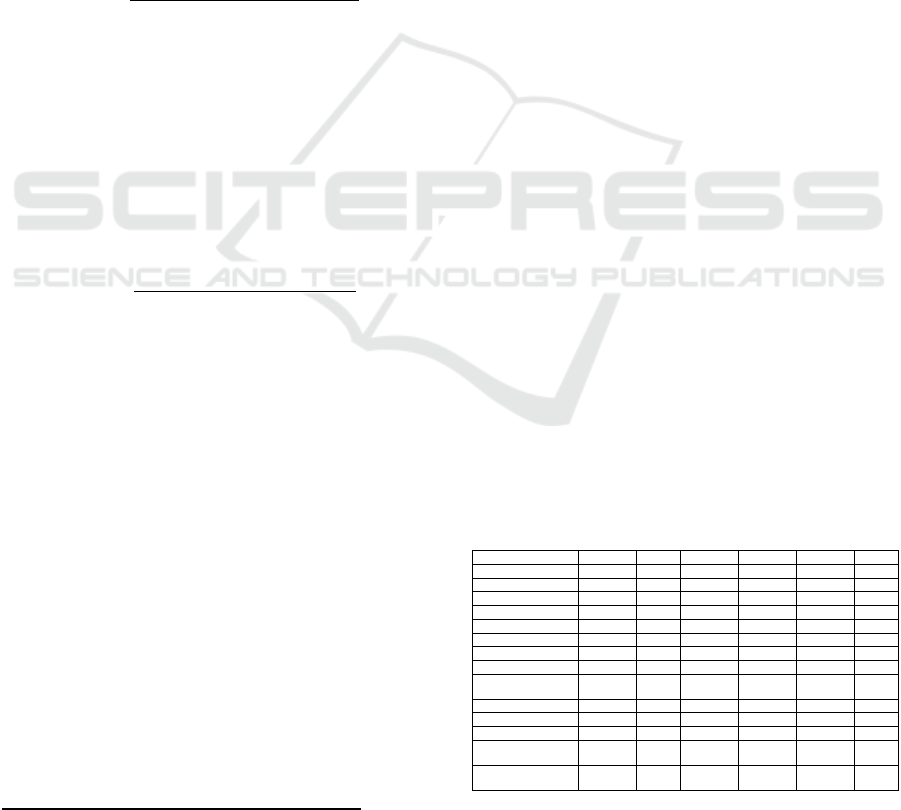
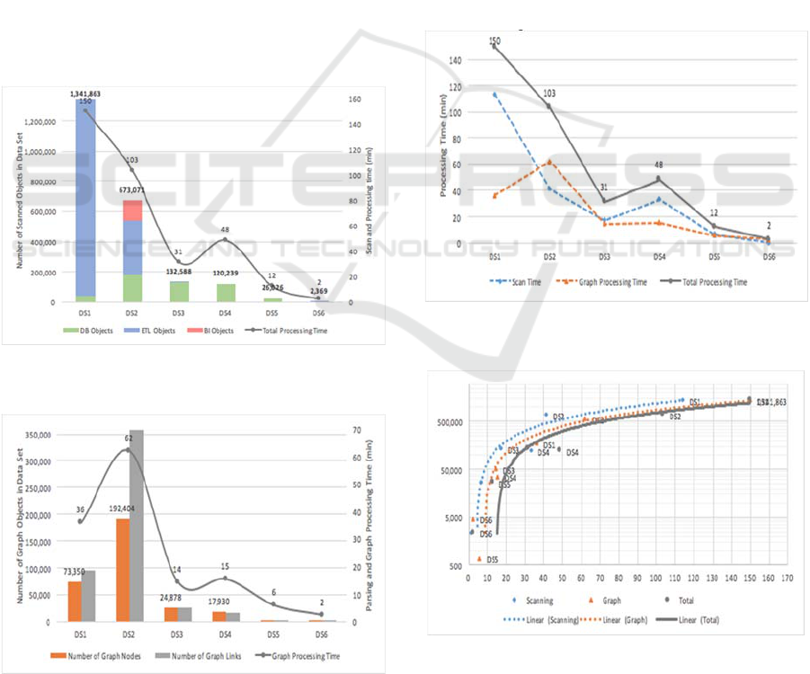
The datasets size, internal structure and
processing time are visible in Figure 2 where longer
processing time of DS4 is related to very big Oracle
stored procedure texts and loading of those to
database.
Figure 2: Datasets size and structure compared to overall
processing time.
Figure 3: Calculated graph size and structure compared to
the graph data processing time.
The initial dataset and the processed data
dependency graphs have different graph structures
(see Figure 3) that do not correspond necessarily to
the initial dataset size. The DS2 has a more integrated
graph structure and a higher number of connected
objects (Figure 4) than the DS1. At the same time the
DS1 has about two times bigger initial row data size
than the DS2.
We have additionally analyzed the correlation of
the processing time and the dataset size (see Figure 4
and Figure 5) and showed that the growth of the
execution time follows the same linear trend as the
size and complexity growth. The data scan time is
related mostly to the initial dataset size. The query
parsing, resolving and graph processing time also
depends mainly on the initial data size, but also on the
calculated graph size (Figure 4). The linear
correlation between the overall system processing
time (seconds) and the dataset size (object count) can
be seen in Figure 5.
Figure 4: Dataset processing time with two main sub-
components.
Figure 5: Dataset size and processing time correlation with
linear regression (semi-log scale).
KDIR 2016 - 8th International Conference on Knowledge Discovery and Information Retrieval
108
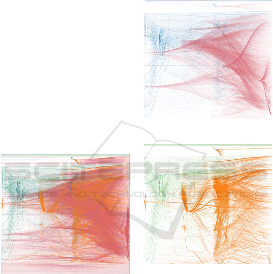
5.2 Dataset Visualization
The Enterprise Dependency Graph examples (Figures
6-8) are an illustration of the complex structure of
dependencies between the DW storage scheme,
access views and user reports. The example is
generated using data warehouse and business
intelligence lineage layers. The details are at the
database and reporting object level, not at column
level. At the column and report level the full data
lineage graph would be about ten times bigger and too
complex to visualize in a single picture. The
following graph from the data warehouse structures
and user reports presents about 50,000 nodes (tables,
views, scripts, queries, reports) and about 200,000
links (data transformations in views and queries) on a
single image (see Figure 6).
The real-life dependency graph examples
illustrate the automated data collection, parsing,
resolving, graph calculation and visualization tasks
implemented in our system. The system requires only
the setup and configuration tasks to be performed
manually. The rest will be done by the scanners,
parsers and the calculation engine.
Figure 6: Data flows (blue, red) and control flows (green,
yellow) between tables, views and reports.
The end result consists of data flows and system
component dependencies visualized in the navigable
and drillable graph or table form. The result can be
viewed as a local subgraph with fixed focus and
suitable filter set to visualize data lineage path from
any sources to single report with click and zoom
navigation features. The big picture of the
dependency network gives the full scale overview
graph of the organization’s data flows. It allows to see
us possible architectural, performance or security
problems.
Figure 7: Data flows between tables, views (blue) and
reports (red).
Figure 8: Control flows in scripts, queries (green) and
reporting queries (yellow) are connecting tables, views and
reports.
6 CONCLUSIONS
We have presented several algorithms and techniques
for quantitative impact analysis, data lineage and
change management. The focus of these methods is
on automated analysis of the semantics of data
conversion systems followed by employing
probabilistic rules for calculating chains and sums of
Discovering Data Lineage from Data Warehouse Procedures
109

impact estimations. The algorithms and techniques
have been successfully employed in several large case
studies, leading to practical data lineage and
component dependency visualizations. We continue
this research by performance measurement with the
number of different big datasets, to present practical
examples and draw conclusion of our approach.
We also considering a more abstract, conceptual
and business level approach in addition to the current
physical/technical level of data lineage representation
and automation.
ACKNOWLEDGEMENTS
The research has been supported by EU through
European Regional Development Fund.
REFERENCES
Anand, M. K., Bowers, S., McPhillips, T., & Ludäscher, B.
(2009, March). Efficient provenance storage over
nested data collections. In Proceedings of the 12th
International Conference on Extending Database
Technology: Advances in Database Technology (pp.
958-969). ACM.
Anand, M. K., Bowers, S., & Ludäscher, B. (2010, March).
Techniques for efficiently querying scientific workflow
provenance graphs. In EDBT (Vol. 10, pp. 287-298).
Benjelloun, O., Sarma, A. D., Hayworth, C., & Widom, J.
(2006). An introduction to ULDBs and the Trio system.
IEEE Data Engineering Bulletin, March 2006.
Buneman, P., Khanna, S., & Wang-Chiew, T. (2001). Why
and where: A characterization of data provenance. In
Database Theory—ICDT 2001 (pp. 316-330). Springer
Berlin Heidelberg.
Cheney, J., Chiticariu, L., & Tan, W. C. (2009). Provenance
in databases: Why, how, and where. Now Publishers
Inc.
Cui, Y., Widom, J., & Wiener, J. L. (2000). Tracing the
lineage of view data in a warehousing environment.
ACM Transactions on Database Systems (TODS),
25(2), 179-227.
Cui, Y., & Widom, J. (2003). Lineage tracing for general
data warehouse transformations. The VLDB Journal—
The International Journal on Very Large Data Bases,
12(1), 41-58.
de Santana, A. S., & de Carvalho Moura, A. M. (2004).
Metadata to support transformations and data &
metadata lineage in a warehousing environment. In
Data Warehousing and Knowledge Discovery (pp. 249-
258). Springer Berlin Heidelberg.
Fan, H., & Poulovassilis, A. (2003, November). Using
AutoMed metadata in data warehousing environments.
In Proceedings of the 6th ACM international workshop
on Data warehousing and OLAP (pp. 86-93). ACM.
Giorgini, P., Rizzi, S., & Garzetti, M. (2008). GRAnD: A
goal-oriented approach to requirement analysis in data
warehouses. Decision Support Systems, 45(1), 4-21.
Heinis, T., & Alonso, G. (2008, June). Efficient lineage
tracking for scientific workflows. In Proceedings of the
2008 ACM SIGMOD international conference on
Management of data (pp. 1007-1018). ACM.
Ikeda, R., Das Sarma, A., & Widom, J. (2013, April).
Logical provenance in data-oriented workflows?. In
Data Engineering (ICDE), 2013 IEEE 29th
International Conference on (pp. 877-888). IEEE.
Missier, P., Belhajjame, K., Zhao, J., Roos, M., & Goble,
C. (2008). Data lineage model for Taverna workflows
with lightweight annotation requirements. In
Provenance and Annotation of Data and Processes (pp.
17-30). Springer Berlin Heidelberg.
Priebe, T., Reisser, A., & Hoang, D. T. A. (2011).
Reinventing the Wheel?! Why Harmonization and
Reuse Fail in Complex Data Warehouse Environments
and a Proposed Solution to the Problem.
Ramesh, B., & Jarke, M. (2001). Toward reference models
for requirements traceability. Software Engineering,
IEEE Transactions on, 27(1), 58-93.
Reisser, A., & Priebe, T. (2009, August). Utilizing
Semantic Web Technologies for Efficient Data Lineage
and Impact Analyses in Data Warehouse Environments.
In Database and Expert Systems Application, 2009.
DEXA'09. 20th International Workshop on (pp. 59-63).
IEEE.
Skoutas, D., & Simitsis, A. (2007). Ontology-based
conceptual design of ETL processes for both structured
and semi-structured data. International Journal on
Semantic Web and Information Systems (IJSWIS),
3(4), 1-24.
Tan, W. C. (2007). Provenance in Databases: Past, Current,
and Future. IEEE Data Eng. Bull., 30(4), 3-12.
Tomingas, K., Tammet, T., & Kliimask, M. (2014), Rule-
Based Impact Analysis for Enterprise Business
Intelligence. In Proceedings of the Artificial
Intelligence Applications and Innovations (AIAI2014)
conference workshop (MT4BD). Series: IFIP
Advances in Information and Communication
Technology, Vol. 437.
Tomingas, K., Kliimask, M., & Tammet, T. (2015). Data
Integration Patterns for Data Warehouse Automation.
In New Trends in Database and Information Systems II
(pp. 41-55). Springer International Publishing.
Vassiliadis, P., Simitsis, A., & Skiadopoulos, S. (2002).
Conceptual modeling for ETL processes. In
Proceedings of the 5th ACM international workshop on
Data Warehousing and OLAP (pp. 14-21). ACM.
Widom, J. (2004). Trio: A system for integrated
management of data, accuracy, and lineage. Technical
Report.
Woodruff, A., & Stonebraker, M. (1997). Supporting fine-
grained data lineage in a database visualization
environment. In Data Engineering, 1997. Proceedings.
13th International Conference on (pp. 91-102). IEEE.
KDIR 2016 - 8th International Conference on Knowledge Discovery and Information Retrieval
110
